Assigning numerical values to categorical (factor) variables is called contrast coding. This need arises when we want to estimate the difference in the dependent variable among different conditions of an independent variable. In other words, we use contrast coding to instruct the Bayesian model to compare the conditional means between different conditions or bundles of conditions.
Treatment, Sum, and Cell Means encoding
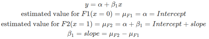
The default contrast coding in R is to rank all string values by alphabetical order (unless you factorise these values and specify the level explicitly), then assign them values from 0 onwards. This is called the treatment contrast.
The condition assigned zero is considered the baseline. In linear regression, the intercept estimates the mean value of the independent variable at the baseline condition. And the slope estimates the difference between the mean of other conditions and the mean of the baseline.
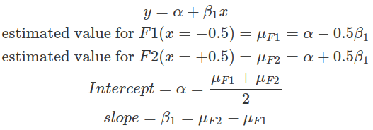
In the sum contrast, conditions are assigned with values centred around zero. This effectively centres each group around the grand mean, that is, the mean of the means of each group. Thus, each group is compared with the grand mean. In balanced datasets where each group contains the same number of observations, the grand mean is the mean of all observations. Whereas, in imbalanced datasets, the grand mean is the weighted mean of all data, and it is biased by groups with less data. This is because the means of every group will be computed first, then the mean of all means. In a two-condition scenario, one can be given -0.5 while the other +0.5. These values are on the same scale as in the treatment contrast case specified above, where the difference between the two conditions is one. This makes interpretations of the intercept and the slope easier. The slope estimates the difference between the two conditions, as in the treatment contrast, and the intercept here estimates the grand mean.
Therefore, treatment contrast compares all other conditions’ means to the baseline condition, whereas the sum contrast compares each condition’s mean against the grand mean (in a two-condition case, this is essentially comparing two group means, as demonstrated above). The selection of which method depends on the hypothesis to be tested. In general, the intercept represents the quantity to compare to, and the slopes (betas) represent differences you want to quantify to test hypotheses.
Alternatively, cell means parameterisation (one-hot encoding) estimates the mean for each condition separately, and no comparison between conditions is made (hence will not be useful for hypothesis testing, such as calculating the Bayes Factor). In brms, fitting a model with such encoding requires explicitly removing the estimate of the intercept (-1+ the factor column). Priors for beta and sigma need to be supplied, and beta is for the intercept (not the slope) per condition. We can then compute differences between conditions using posterior samples drawn from the model fitting result, and assess the means and 95% intervals of these differences (the mean differences should be very close to the slopes estimated with the above contrasting methods). However, as posterior distributions depend on both the prior distribution and the data, if the prior used is very informative, then the mean differences calculated using the posterior would be different from the above contrasting methods. This encoding method provides flexibility; however, it can not be used to reject the null hypothesis, where an explicit hypothesis test by the Bayes Factor is needed.
packs=c("brms","rstan","bayesplot","dplyr","purrr","tidyr","ggplot2","ggpubr","extraDistr","sn","hypr","lme4","rootSolve","bcogsci","tictoc","MASS")
lapply(packs, require, character.only = TRUE)

select = dplyr::select
extract = rstan::extract
filter=dplyr::filter

### read in data ###
df_contrasts1

###############################################################
### fit with default R contrast coding-- treatment contrast ###
###############################################################
# this shows the default contrasting
contrasts(df_contrasts1$F)

fit_F_treatmentc = brm(output ~ F,
             data = df_contrasts1,
             family = gaussian(),
             prior = c(prior(normal(0, 2), class = Intercept),
                       prior(normal(0, 2), class = sigma),
                       prior(normal(0, 1), class = b)))

fit_F_treatmentc

# the intercept is the mean of F1, and FF2 is the mean(F2)-mean(F1)
fixef(fit_F_treatmentc)

# look at the mean for F1, 0.8
df_contrasts1 %>%
  filter(F=="F1") %>%
  select(output) %>%
  colMeans()

# look at the mean for F2, 0.4
df_contrasts1 %>%
  filter(F=="F2") %>%
  select(output) %>%
  colMeans()

contrasts(df_contrasts1$F)


####################
### sum contrast ###
####################
# assign contrasts to data
contrasts(df_contrasts1$F)=c(-0.5,0.5)
contrasts(df_contrasts1$F)
fit_F_sumc = brm(output ~ F,
                   data = df_contrasts1,
                   family = gaussian(),
                   prior = c(prior(normal(0, 2), class = Intercept),
                             prior(normal(0, 2), class = sigma),
                             prior(normal(0, 1), class = b)))
fixef(fit_F_sumc)

###################################
### Cell Means Parameterisation ###
###################################
# re-read in data
df_contrasts1

# directly fitting the model
fit_F_cellmeansc = brm(output ~ -1 + F,
               data = df_contrasts1,
               family = gaussian(),
               #only two priors, b is for intercepts for each condition
               prior = c(prior(normal(0, 2), class = sigma),
                         prior(normal(0, 2), class = b)))

fixef(fit_F_cellmeansc)

# draw the posterior samples
fit_F_cellmeansc_post=as_draws_df(fit_F_cellmeansc)
# calculate difference
fit_F_cellmeansc_post_diff=fit_F_cellmeansc_post %>%
  mutate(f1_f2_diff=b_FF2-b_FF1)
# compute the mean and 95% CI (mean value should be similar to above slope, however also dependent on strength of priors)
c(mean=mean(fit_F_cellmeansc_post_diff$f1_f2_diff),quantile(fit_F_cellmeansc_post_diff$f1_f2_diff,p=c(0.025,0.975)))
Hypothesis to Contrast Matrix
In more complex scenarios, such as multiple comparisons with more than two conditions, contrast coding depends on the hypothesis and often requires specialised packages to encode the contrast matrix.
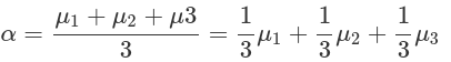
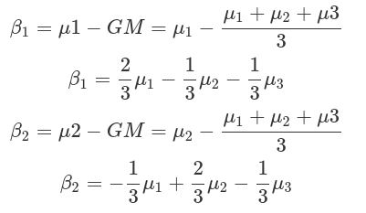
Assume we have three drugs and their corresponding survival durations. We want to test whether drug1 has a shorter survival time than the grand mean, and whether drug2 has a longer time. We also want to quantify the differences between the two drugs and the grand mean. The fractions (weights), in front of the mean of each condition, derived from the comparisons we want to make (betas), indicate how to combine conditions to generate contrasts to be used in a linear regression model.
Contrast encoding needs to fit the comparisons we want to make. And contrasts can be generated from these comparisons:
- Define the comparisons (each comparison corresponds to one beta)
- Compose the Hypothesis Matrix.
Extract weights in front of each condition, as well as for the intercept, into a data frame with conditions as columns, comparisons as rows. Weights for the intercept (alpha) should be encoded in the first row. This data frame is called the Comparison Matrix or Hypothesis Matrix. - Apply Generalised Matrix Inverse to the Hypothesis Matrix to obtain the Contrast Matrix (bcogsci::ginn2() or MASS::ginv()).
The Contrast Matrix has conditions as rows and comparisons as columns. The result shown in the example below is a Sum Contrast where +1 labels the condition to be compared with the grand mean; whereas -1 labels the condition that will never be compared. - Assign the Contrast Matrix to the factors. Then fit into the Bayesian model.
Before assigning contrasts to the factors by contrasts() function, the contrast for intercept (first column from the contrast matrix) should be removed, because brm automatically adds this in. The results show the estimate of the grand mean (intercept), and comparisons (betas) as you defined in the hypothesis matrix.
We can also use the hypr package to automatically convert comparisons, defined by the factor levels, to contrasts. The hypr package uses “~” to define differences, other than “-“. In the output, comparisons are addressed as “null hypotheses”, as by frequentists. In the Bayesian framework, these are comparisons between conditional means.
#################################################
### from Hypothesis Matrix to Contrast Matrix ###
#################################################

### manually derive contrasts to demonstrate the procedure ###
# read in data
df_contrasts2

#1,2 hypothesis matrix, comparisons as rows
hypoM=rbind(inter=c(drug1=1/3,drug2=1/3,drug3=1/3),
            b1=c(drug1=2/3,drug2=-1/3,drug3=-1/3),
            b2=c(drug1=-1/3,drug2=2/3,drug3=-1/3))
hypoM
#fractions is a function from package MASS
fractions(hypoM)

#3 contrast matrix
contM=ginv2(hypoM)
contM

# use R package to generate sum contrast ###
# just need to manually combine with intercept, 3 indicates three conditions
contM_R=cbind(1,contr.sum(3))
contM_R

#4 assign contM to factors in data, and fit in model
# make sure the column for intercept is removed from the contrasts, because brm will automatically add it in.
# make sure the original data's conditions are in factors
contrasts(df_contrasts2$drug)=contM[,2:3]
df_contrasts2
contrasts(df_contrasts2$drug)


fit_sum_contM=brm(duration~drug,
                  data=df_contrasts2,
                  family=gaussian(),
                  prior=c(prior(normal(450,100),class=Intercept),
                          prior(normal(0,100),class=sigma),
                          prior(normal(0,100),class=b)))
fixef(fit_sum_contM)

### use the hyper package ###
#just define your comparisons (no need for intercept)
# CAUSION, use "~" instead of "-"
contM_hypr=hypr(b1=drug1~(drug1+drug2+drug3)/3,
                b2=drug2~(drug1+drug2+drug3)/3,
                levels=c("drug1","drug2","drug3"))

# this will generate transposed hypothesis matrix (conditions as rows, comparisons as columns as in contrast matrix) and contrast matrix
contM_hypr
# use contr.hypothesis to retrieve the contrast matrix
contr.hypothesis(contM_hypr)

# assgin contrasts to factors, there are only comparisons no intercept, brm will automatically adds contrasts for intercept.
contrasts(df_contrasts2$drug)=contr.hypothesis(contM_hypr)
contrasts(df_contrasts2$drug)
Repeated difference, Helmert, Polynomial contrast and monotonic relationship
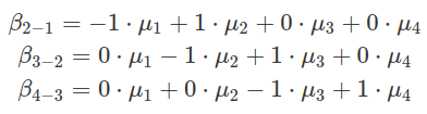
There are other types of contrasts. One is called repeated differences, in which comparisons are made between neighbouring levels. For example, each level is compared with the level above. And the mean of the first one to compare is estimated as the intercept, which is the second level. In the following example, there are four conditions (levels), named from F1 to F4. The contrast matrix can be generated by either hypr package or contr.sdif() from MASS. The comparison results of F2 to F1, F3 to F2 and F4 to F3 are encoded in the estimates of three beta values, as shown in the example below.
######################################
### repeated differences contrasts ###
######################################

# read in data
df_contrasts3

# define contrast by hypr
repeatedD_contM_hypr=hypr(f2v1=F2~F1,
                          f3v2=F3~F2,
                          f4v3=F4~F3,
                          levels = c("F1","F2","F3","F4"))
repeatedD_contM_hypr

# verify above contrast matrix by R function
fractions(contr.sdif(4))

# assign contrasts to levels of the factor
contrasts(df_contrasts3$F)=contr.hypothesis(repeatedD_contM_hypr)
contrasts(df_contrasts3$F)

# fit the model
fit_repeatedD=brm(outcome~F,
                  data=df_contrasts3,
                  family=gaussian(),
                  prior=c(prior(normal(20,40),class=Intercept),
                          prior(normal(0,35),class=sigma),
                          prior(normal(0,20),class=b)))

fixef(fit_repeatedD)

# figure out which level's mean is intercept estimating?
# average: F1 10, F2 20, F3 10, F4 40
# so the intercept is actually F2 !!! (not F1)
df_contrasts3 %>%
  filter(F=="F4") %>%
  select(outcome) %>%
  colMeans()
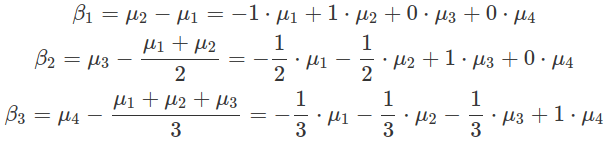
In Helmert contrasts, each level is compared to the mean of all levels above. The hypr implementation of this contrast is more intuitive than contr.helmert(), which generates a scaled version. The hypr generated contrasts correspond to the real differences between levels, other than the scaled version of them. This intuitive approach makes setting up priors and interpreting posteriors easier. The intercept in model fitting results estimates the mean for the first level shown in the comparison formula, which is the second level.
########################
### Helmert Contrast ###
########################

# use hypr pacakge to manually implement the contrast
# the generated contrasts directly correspond to real differences between levels.
helmertC_hypr=hypr(b1=F2~F1,
                   b2=F3~(F1+F2)/2,
                   b3=F4~(F1+F2+F3)/3,
                   levels=c("F1","F2","F3","F4"))
helmertC_hypr

#use contr.helmert to implement. 4 indicates 4 levels.
# in the generated contrasts, b1 is hypr generated b1x2, b2 is hypr b2x3, and b3 is b3x4. This makes the prior setting tricky
contr.helmert(4)

#assign contrast and fit model
contrasts(df_contrasts3$F)=contr.hypothesis(helmertC_hypr)
contrasts(df_contrasts3$F)

fit_helmert=brm(outcome~F,
                  data=df_contrasts3,
                  family=gaussian(),
                  prior=c(prior(normal(20,40),class=Intercept),
                          prior(normal(0,35),class=sigma),
                          prior(normal(0,20),class=b)))

fixef(fit_helmert)
After assigning the contrasts to levels, while fitting the linear regression model, the contrast matrix is first converted into a model matrix, which essentially maps numerical values encoded by contrasts onto observations (data point on each row) based on their corresponding levels. Multiple comparisons (multiple betas or multiple columns in the contrast matrix) expand the data matrix by multiple columns, each of which is a translation from the level of data to one set of contrasts corresponding to one comparison (or one beta). These columns are treated as different predictors (covariates) in a linear model, having their separate betas. And the fitted posterior results on betas are interpreted as the comparison outcome. The summation in a linear model among all predictors does not necessarily mean their effects are additive. If these contrasts (comparisons) are orthogonal, they are not interacting with each other.
####################################
### what model matrix looks like ###
####################################
# assign contrast matrix to levels
contrasts(df_contrasts3$F)=contr.hypothesis(helmertC_hypr)
contrasts(df_contrasts3$F)

# model matrix showing the expansion of the columns each correspond to a comparison, plus the intercept
covariates=model.matrix(~1+F,df_contrasts3)

# we can use the model.matrix above to expand the data mannually and demonstrate it is the same concept as assign contrasts, then fit the model
df_contrasts3[,c("b1","b2","b3")]=covariates[,2:4]
df_contrasts3

# fit the model using b1,b2,b3 as covariates or separate predictors
#   the following results are the same as fit_helmert
fit_helmert2=brm(outcome~b1+b2+b3,
                 data=df_contrasts3,
                 family=gaussian(),
                 prior=c(prior(normal(20,45),class=Intercept),
                         prior(normal(0,40),class=sigma),
                         prior(normal(0,20),class=b)))

fixef(fit_helmert2)
fixef(fit_helmert)
Sometimes, different factor levels have a joint linear or non-linear effect on the dependent variable. The difference between any two levels is difficult to detect than when combining all levels. For instance, in some linear relationships, we expect an increase in the factor level to result in an increase or decrease in the dependent variable. And there are shared trends (parameters) collectively among levels. This relationship can be assessed by the polynomial contrasts. As the number of levels increases, this polynomial relationship can be extended to higher orders. For example, for a four-level factor, we can detect linear (F.L), quadratic (F.Q), and cubic (F.C) relationships. The intercept estimates the mean for the second level factor.
It is unclear how scaling is applied to the contrasts defined by contr.poly() function. Therefore, it is tricky to define priors for beta, and the posteriors are difficult to interpret. It is better to set up the linear contrasts manually, then derive the higher-order contrasts accordingly. Before applying these contrasts to factor levels, it is advisable to orthogonalize the highly correlated contrasts (e.g. linear and cubic contrasts) by extracting residuals from a linear model between the two.
################################
### Polynormial relationship ###
################################
df_contrasts3
### contr.poly() ###
# define and assign contrasts by contr.poly(), 4 shows the number of levels.
contrasts(df_contrasts3$F)=contr.poly(4)

contrasts(df_contrasts3$F)

# fit the model
fit_polynomial=brm(outcome~F,
                   data=df_contrasts3,
                   family=gaussian(),
                   prior=c(prior(normal(20,45),class=Intercept),
                           prior(normal(0,20),class=sigma),
                           prior(normal(0,20),class=b)))
fixef(fit_polynomial)

### manual define (preferred) ###
# define the linear relationship with 1 unit define as level separation, and all levels are spread from zero
poly_man=data.frame(linear=c(F1=-3,
                             F2=-1,
                             F3=1,
                             F4=3)/2)

# define quadratic (square up the level, then spread them from the mean) and cubic (cube the level, then spread from mean) relationship
poly_man$quadratic=poly_man$linear^2-mean(poly_man$linear^2)
poly_man$cubic=poly_man$linear^3-mean(poly_man$linear^3)

# as can be judged from the sign the levels, the linear and cubic relationship are correlated, you need to orthogonalize the two.
# fitting a linear relationship, finding the correlation between cubic and linear contrasts, then use residuals() or resid() to extract the model residual from correlated cubic and linear relationship
poly_man$cubic=residuals(lm(cubic~linear,poly_man))

poly_man

# assign the contrasts
contrasts(df_contrasts3$F)=as.matrix(poly_man)
contrasts(df_contrasts3$F)


# fit the model
fit_polynomial_man=brm(outcome~F,
                   data=df_contrasts3,
                   family=gaussian(),
                   prior=c(prior(normal(20,45),class=Intercept),
                           prior(normal(0,20),class=sigma),
                           prior(normal(0,20),class=b)))

# the result is more interpretable
fixef(fit_polynomial_man)
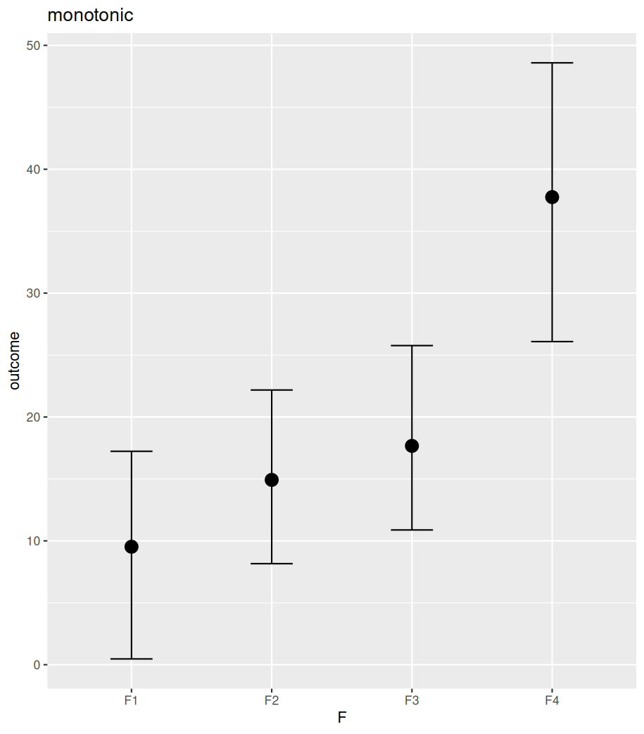
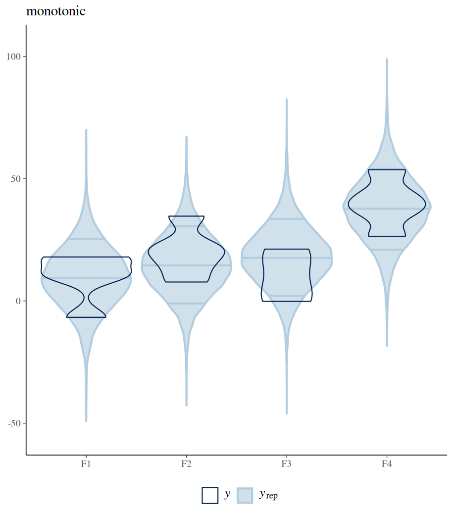
Instead of setting up contrasts, we can assume a monotonic (one-directional) trend across ordered levels of a factor. Based on this assumption, we can directly estimate the average increase or decrease in the independent variable between all neighbouring levels, as well as their corresponding ratios of contribution to the average change. To define this in brms, factorise levels in a desirable order (e.g. factor(…, ordered=TRUE, levels=c()) and use mo() when setting up the model relationship. In the fitting result, the Intercept estimates the mean of the first level; the regression coefficient shows the average increase or decrease in the independent variable with each level; and the simplex parameter indicates the ratio of the overall change associated with every pair of neighbouring levels.
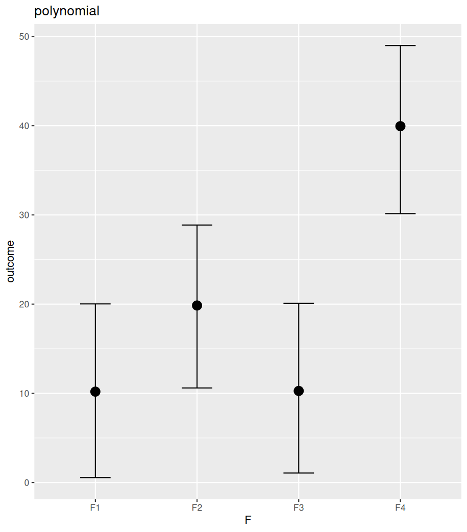
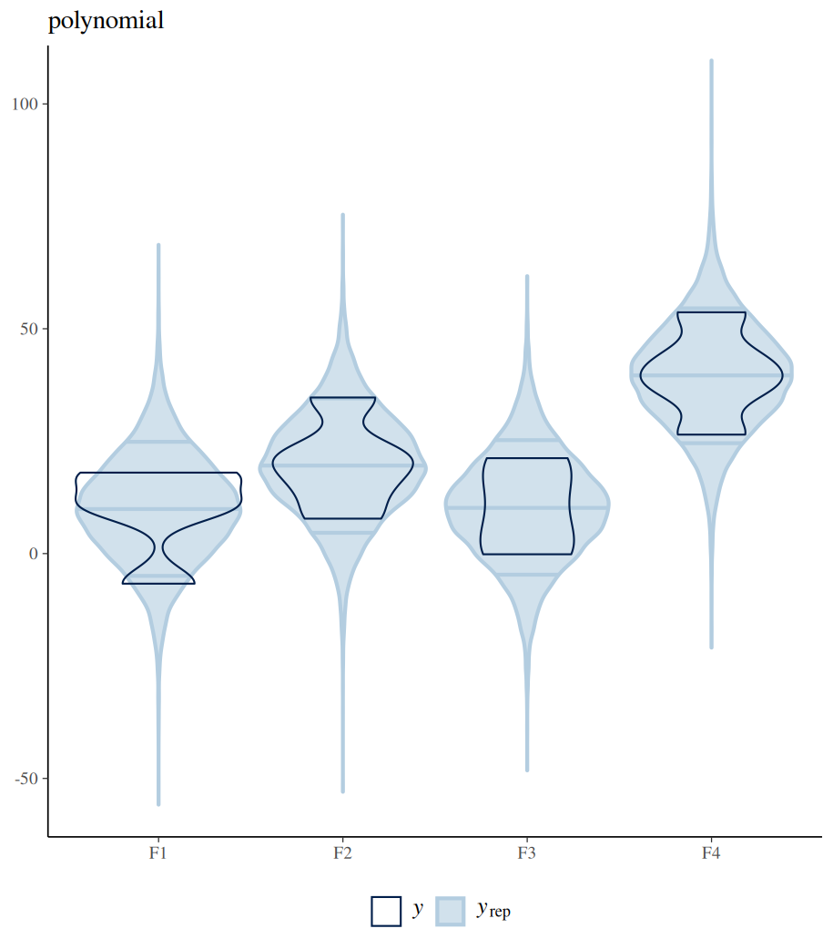
The difference between polynomial and monotonic relationships is that the polynomial coefficient is obtained by drawing a line sitting in the middle among all differences between the means of neighbouring levels. These differences can be increases or decreases. Whereas a monotonic relationship assumes and forces one-directional change, regardless of the real differences among these means. The following example shows the differences between these two models in their estimated conditional means (by conditional_effects()). Further posterior sampling and data comparison (pp_check()) demonstrate how the monotonic assumption violates the real differences between levels. Despite all these, the monotonic model is useful when specific differences between conditions are not of interest, but the overall monotonic effect is.
#################
### monotonic ###
#################
# define ordered factor for F
df_contrasts3$F=factor(df_contrasts3$F, ordered=TRUE,levels=c("F1","F2","F3","F4"))
df_contrasts3

# fit the model while using mo() to define monotonic relationship
fit_mono=brm(outcome~1+mo(F),
             data=df_contrasts3,
             family=gaussian(),
             prior=c(prior(normal(20,45),class=Intercept),
                     prior(normal(0,20),class=sigma),
                     prior(normal(0,20),class=b)))
fit_mono

### compare polynomial and monotonic relationship model coefficients estimations ###
# model estimated conditional means
conditional_effects(fit_polynomial_man)
conditional_effects(fit_mono)
plot(conditional_effects(fit_polynomial_man), plot=FALSE)[[1]]+ggtitle("polynomial")
plot(conditional_effects(fit_mono), plot=FALSE)[[1]]+ggtitle("monotonic")

# posterior sampling and comparison with real data
pp_check(fit_polynomial_man,type="violin_grouped",group = "F",y_draws="points")+
  theme(legend.position = "bottom")+
  coord_cartesian(ylim = c(-55, 105)) +
  ggtitle("polynomial")

pp_check(fit_mono,type="violin_grouped",group = "F",y_draws="points")+
  theme(legend.position = "bottom")+
  coord_cartesian(ylim = c(-55, 105)) +
  ggtitle("monotonic")
What makes a good contrasts?
For n conditions, there can only be n-1 independent comparisons. This is because of the estimation of the intercept. In a two-factor system, each factor has n1 and n2 levels. There are n1 x n2 – 1 contrasts.
Contrasts should not be colinear; in other words, contrasts should not be in a linear relationship, and should not be able to generate one another via linear combinations. Comparisons should capture independent information. To generate good contrasts, one should bear the following three points in mind:
- Encode orthogonal contrasts for mutually exclusive comparisons
- Answer research questions
- Scale contrasts properly to facilitate prior definitions and posterior interpretations
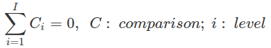
Most contrasts mentioned here, except the treatment contrast, are centred, that is, in the contrast matrix, the sum of all coefficients for different levels of one comparison equals zero (colSums=0).
The coefficients in a hypothesis matrix are always centred, even for the treatment contrast. The only exception is the coefficients for the intercept that always sum to one, to ensure that after applying the generalised matrix inverse, these coefficients become constants (all are 1).
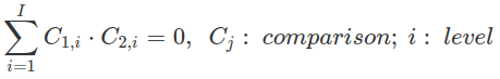
Two of the centred contrasts are orthogonal to each other if the sum of products between contrasts (comparisons) for the same level equals zero.
Orthogonal contrasts are not correlated (their correlation coefficient equals 0). This is another way to judge whether two contrasts are orthogonal. In the following example, we encode a two-factor (F1, F2) two-level (1 and -1) design (four combinations and one interaction) using the sum contrasts. Any pair of these contrasts is orthogonal to each other, which is indicated by the zeros of the off-diagonal elements in the correlation matrix (cor(), off-diagonal is the line running from bottom left to top right). However, contrasts generated for a multi-level factor by sum contrast, treatment contrast or repeated contrast are not orthogonal.
When the generalised inverse of a matrix is computed, orthogonal contrasts are inverted independently, meaning that one does not affect the outcome of another. In this case, generalised inversion only results in a scaled version of the hypothesis matrix.
Intercept should be included when computing the generalised matrix inversion for non-centred contrasts (e.g. the treatment contrasts). This is because only the centred contrasts are orthogonal to the intercept (as intercepts are 1s, when multiplying with centred contrasts, the sum of these products is zero), hence they can be inverted independently (then add all the 1s for the intercept after the inversion). However, for non-centred contrasts, as they are not orthogonal to the intercept, the intercept needs to be inverted with all contrasts. This will ensure the intercept and all contrasts (slopes) are set up correctly.
#########################
### centered contrast ###
#########################
# treatment contrast is not centered
colSums(contr.treatment(4))

# other contrasts are centered
colSums(contr.sum(4))
colSums(contr.poly(4))
colSums(contr.helmert(4))
colSums(contr.sdif(4))


############################
### orthogonal contrasts ###
############################
sum_2level = cbind(F1 = c(1, 1, -1, -1),
              F2 = c(1, -1, 1, -1),
              F1xF2 = c(1, -1, -1, 1))
sum_2level

# look at correlations between any pair of columns, which indicates the orthogonal relationship
cor(sum_2level)

# however contrasts for multi-level factor encoded by sum contrasts, repeated difference and treatment contrats are not orthogonal
cor(contr.sum(4))
cor(contr.sdif(4))
cor(contr.treatment(4))

cor(contr.helmert(4))


##############################################################
### intercept should be considered for uncentred contrasts ###
##############################################################
# for uncetered contrasts such as treatment contrasts, intercept should be included
# the following two getting the same contrasts, whether by hypr package or contr.treatment
hypr(int=a~0,b1=b~a,b2=c~b, levels=c("a","b","c"))
contr.treatment(c("a","b","c"))

# if we do not consider intercept, we obtain completely different contrasts from above.
#   as the following getting the same contrasts, which means the intercept for both is actually the grand mean
hypr(b1=b~a,b2=c~b)
hypr(int=(a+b+c)/3~0,b1=b~a,b2=c~b)
Calculate condition means from contrasts
When fitting a model without contrasts, for instance, the cell means parametrisation, we essentially compute the condition mean for each level of a factor (by ignoring the Intercept in the brm model). Afterwards, we can make comparisons between levels from posterior sampling of these condition means. Likewise, when fitting a model with contrasts, we can calculate condition means from posterior sampling of these contrasts. Each row of the contrast matrix, corresponding to a level, provides a formula to calculate the condition mean for the specific level by combining posteriors of contrasts and the intercept. Furthermore, the mean and 95% credible intervals of these condition means can be computed, and additional comparisons can be made post hoc. For example, we can obtain the grand mean based on all the posterior samples of the condition means and compare conditions to the grand mean that have not been conducted during model fitting. In fact, conditional_effects() function from brms can compute and plot these condition means automatically.
In Bayesian modelling, it is important to understand that obtaining the posterior distribution of a contrast (or a comparison) is not evidence for the effect or the difference. It is only the Bayesian Factor that can show whether an evidence of effect is present or not, and it also shows the magnitude.
###########################################
#### from contrasts to condition means ####
###########################################
## read in the data
data("df_contrasts2")
head(df_contrasts2)

df_contrasts2=df_contrasts2 %>%
  mutate(drug=case_when(F=="adjectives"~"drug1",
                        F=="nouns"~"drug2",
                        F=="verbs"~"drug3",
                        TRUE~"durgUnknown")) %>%
  mutate(drug=factor(drug)) %>%
  rename("duration"="DV") %>%
  select(id,drug,duration)


# data
df_contrasts2

## three level sum contrasts (two contrasts) for drug1 and drug3 compare with grand mean
sum_hypr=hypr(b1=drug1~(drug1+drug2+drug3)/3,
              b2=drug3~(drug1+drug2+drug3)/3,
              levels=c("drug1","drug2","drug3"))
contr.hypothesis(sum_hypr)

# use contrasts to fit model
contrasts(df_contrasts2$drug)=contr.hypothesis(sum_hypr)
df_contrasts2
contrasts(df_contrasts2$drug)


fit_sum_hypr=brm(duration~drug,
                  data=df_contrasts2,
                  family=gaussian(),
                  prior=c(prior(normal(450,100),class=Intercept),
                          prior(normal(0,100),class=sigma),
                          prior(normal(0,100),class=b)))

fixef(fit_sum_hypr)

# posterior sampling for contrasts b1 and b2
df_posterior_sumhypr=as_draws_df(fit_sum_hypr)
df_posterior_sumhypr

# use coefficients in contrast matrix to finds posterior condition mean for drug1 and drug3
df_condition_means=df_posterior_sumhypr %>%
  mutate(drug1cm=b_Intercept+1*b_drugb1+0*b_drugb2,
         drug2cm=b_Intercept+(-1)*b_drugb1+(-1)*b_drugb2,
         drug3cm=b_Intercept+0*b_drugb1+1*b_drugb2) %>%
  as.data.frame() %>%
  select(drug1cm,drug2cm,drug3cm)

df_condition_means

# calculate mean and 95% CI
df_condition_means %>%
  pivot_longer(cols=everything(),
               names_to="drug",
               values_to="condition_mean") %>%
  group_by(drug) %>%
  summarise(mean=mean(condition_mean),
            "2.5%"=quantile(condition_mean,p=0.025),
            "97.5%"=quantile(condition_mean,p=0.975))

# plot
df_condition_means %>%
  pivot_longer(cols=everything(),
               names_to="drug",
               values_to="condition_mean") %>%
  ggplot()+
  geom_boxplot(aes(x=drug,y=condition_mean))

# directly use conditional_effects([model_fitting_result])
  # robust=FALSE make it show mean, other than median
  # the following will plot
conditional_effects(fit_sum_hypr, robust=FALSE)

  #the following will produce mean and 95% CI
conditional_effects(fit_sum_hypr, robust=FALSE)[]

# posterior sample calculated condition means can be used to make further comparison, e.g. compare drug2 with grand mean
drug2_vs_mean=df_condition_means %>%
  mutate(drug2_vs_mean=drug2cm-(drug1cm+drug2cm+drug3cm)/3) %>%
  select(drug2_vs_mean)
drug2_vs_mean

c(mean=mean(drug2_vs_mean$drug2_vs_mean),"2.5%"=quantile(drug2_vs_mean$drug2_vs_mean,p=0.025),"97.5%"=quantile(drug2_vs_mean$drug2_vs_mean,p=0.975))
