Bayesian Hierarchical Model

Data is often grouped by similarities that arise from repeated measurements for each subject or experimental item. This structure can be represented as hierarchies. This type of model is known as a hierarchical model, multi-level model, mixed model, or partial pooling model.

Exchangeability

The Bayesian hierarchical model is based on the assumption of exchangeability. This means that we can rearrange the subjects (e.g. shuffle the index of the group variable) without losing any information, and the joint probability distribution will remain unchanged. This implies that these subjects are identically distributed, originating from the same prior distribution, with none holding a unique prior. Additionally, the observations for each subject (or within each group) are also considered exchangeable.

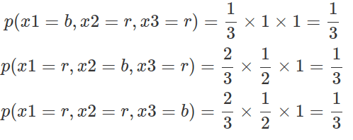
The concepts of exchangeability and frequentists’ notion of “identical and independence” are distinct. If events are identical and independent, they are considered exchangeable; whereas exchangeability only implies identical distribution, not necessarily independence. Consider a box containing one black ball and two red balls. When retrieving balls without replacement, the outcome of each retrieval depends on the previous ones, resulting in dependence. Nonetheless, the probability of getting three balls in any order remains the same. Specifically, there are three possible sequences of events: black, red, red; red, black, red; and red, red, back. As demonstrated below, changing the order of these events (X) yields the same probability. Furthermore, at each retrieval event (any steps Xn of all possible sequences), the likelihood of drawing a red ball is always 2/3, while the probability of drawing a black ball is 1/3.

Predictors, whether at the observation level or the cluster level, are designed to capture all information that is not exchangeable. When all predictors are factored out, the observations become interchangeable, which means their interchangeability is conditional on these predictors. Bayesian hierarchies, or exchangeability within and across clusters, enable us to generalise about the underlying population, as long as the population is randomly sampled.

Completing pooling, no pooling, and hierarchical model

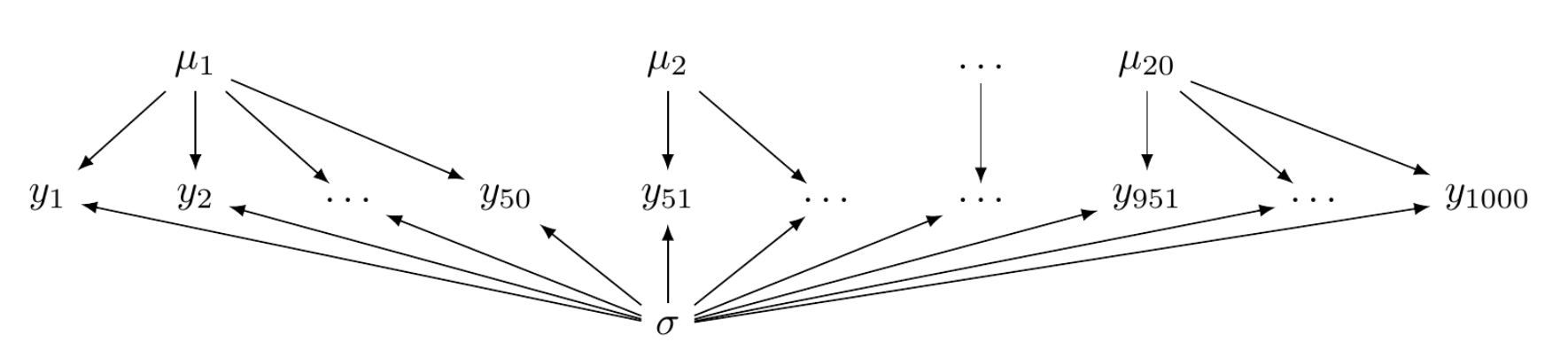
According to the representation theorem, if random variables—such as those representing sequential events shown above—are exchangeable, then the prior distributions regarding these variables are necessary consequences. In other words, these variables are sampled from the same distribution. For instance, we can assume that the mean measurements for each group variable share a single prior distribution. This creates a hierarchical structure, allowing group-level parameters to share common priors, which can be defined by hyper-parameters. See the example below.

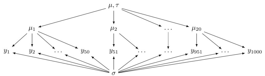
Hyper-parameters define the overall mean and variability at the group level, which in turn influences the mean for each individual group. Hence, the mean for each group is affected not only by a common distribution but also by observations from other groups. Each group’s mean borrows strength from the grand mean of all groups. As a result, in a sparse dataset where some subjects have missing data, their means are significantly reliant on the group mean.

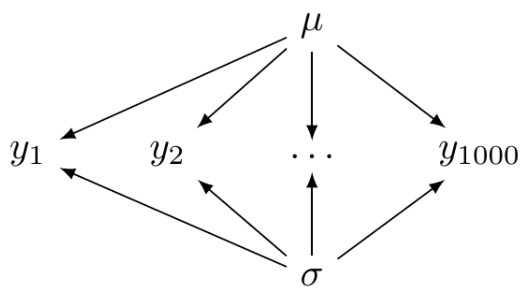
Hierarchical models fall between two extremes: complete pooling (figure below left) and no pooling (figure below right). The complete-pooling model assumes that all observations are independent and drawn from a single distribution, without considering any clusters or groups. This approach is also known as the fixed effects model, as all parameters are fixed and do not vary across different groups. The syntax used by brms is the same as that for general linear models.

In the no-pooling model, observations are not independent but clustered into groups. Those groups themselves are independent. Hence, within a group, observations are assumed to be sampled from an independent distribution. There is no shared distribution nor shared parameters among these groups. Fitting such a model by brms requires eliminating the common Intercept and factorising the group variable. No-pooling models force estimations for each group and result in the same number of intercepts (alphas) and slopes (betas, if the effects of independent variables are to be estimated) as the number of groups. In practice, only one prior distribution is needed and shared among all the betas (by eliminating the ‘coef’ parameter). While the prior knowledge about these betas is the same, they remain independent from one another.

No-pooling models are not recommended because they might underfit when there is insufficient data for some groups or overfit when there is too much data for others.

Hierarchical model by brms

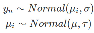
To establish a hierarchy, the brms package requires defining group variables and setting priors for hyperparameters. In the provided example, the hyperparameters mu and tau correspond to the Intercept and sd in brms syntax, respectively. Additionally, individual-level parameters, such as sigma, align with the sigma in brms. Furthermore, posterior sampling illustrates how each group deviates from the overall mean. Hierarchies can also be built for sigma or other parameters in the likelihood function.

packs=c("brms","rstan","bayesplot","dplyr","purrr","tidyr","ggplot2","ggpubr","extraDistr","sn","hypr","lme4","rootSolve","bcogsci","tictoc")
lapply(packs, require, character.only = TRUE)

select = dplyr::select
extract = rstan::extract
filter=dplyr::filter

######################
### synthetic data ###
######################
# backbone
n_sub=20
n_obs=30
n=n_sub*n_obs
df=tibble(row=1:n,
          sub=rep(1:n_sub,each=n_obs))
df

## complete pooling, all data from one distribution
mu=100
sd=5
df_cp=mutate(df,y=rnorm(n=n,mean=mu,sd=sd))
df_cp

df_cp_fit=brm(y~1,
               data=df_cp,
               family=gaussian(),
               prior=c(prior(normal(50,100),class=Intercept),
                       prior(normal(10,20),class=sigma)))

df_cp_fit
plot(df_cp_fit)

## no pooling, all subj has its own distribution
mus=runif(20,min=0,max=100)
sd=5
df_np=mutate(df,y=rnorm(n=n,mean=mus,sd=sd)) # total samples will be n, and evenly ditributed between all means

# when fitting no-pooling, set intercept as 0 and factorize the variable for groups
#   do not set prior for Intercept, but for all individual intercept per group, labelled as b
df_np_fit=brm(y~0+factor(sub),
              data=df_np,
              family=gaussian(),
              prior=c(prior(normal(50,100),class=b),
                      prior(normal(10,20),class=sigma)))
df_np_fit
df_np_fit %>% posterior_summary() #display the posterior mean and 95% credible interval for each group

## hierarchical model (partial pooling model)
mu=100
sd=5
tau=10

mui=rnorm(n_sub,mean=mu,sd=tau)
df_h=mutate(df,y=rnorm(n,mui,sd=sd))

df_h_fit=brm(y~1+(1|sub),
             data=df_h,
             prior=c(prior(normal(50,100),class=Intercept),
#sigmal models within group variation
                     prior(normal(5,10),class=sigma),
#sd models group-level variation tau
                     prior(normal(5,10),class=sd)),
             #increase iter, and adapt_delta to avoid none convergence
             iter=5000,
             control=list(adapt_delta=0.9,
                          max_treedepth=15)
             )

#in the result, "sd(Intercept)" refers to tau showing group-level variation, "sigma" shows within group variation
df_h_fit 
#this will show all the summary of posterior estimations including each group's adjustments to the Intercept, names as r_sub[No.,Intercept], remember mu_i=mu+adjustment
df_h_fit %>% posterior_summary() 

# posterior sampling of all group level adjustments
#   sample are organized as columns for variables, rows for samples.
#   for the following, columns for each group, rows are samples
ui_adjusts=df_h_fit %>% 
  as_draws_df() %>% 
  select(starts_with("r_sub"))
         
# extract the Intercept
u=as_draws_df(df_h_fit)$b_Intercept
u

# u+ui_adjust, each colunm of ui_adjust add u
ui_post=u+ui_adjusts
ui_post

#calculate column means as mean of posterior sample for each column
colMeans(ui_post) %>% unname()

Hierarchical model with one predictor

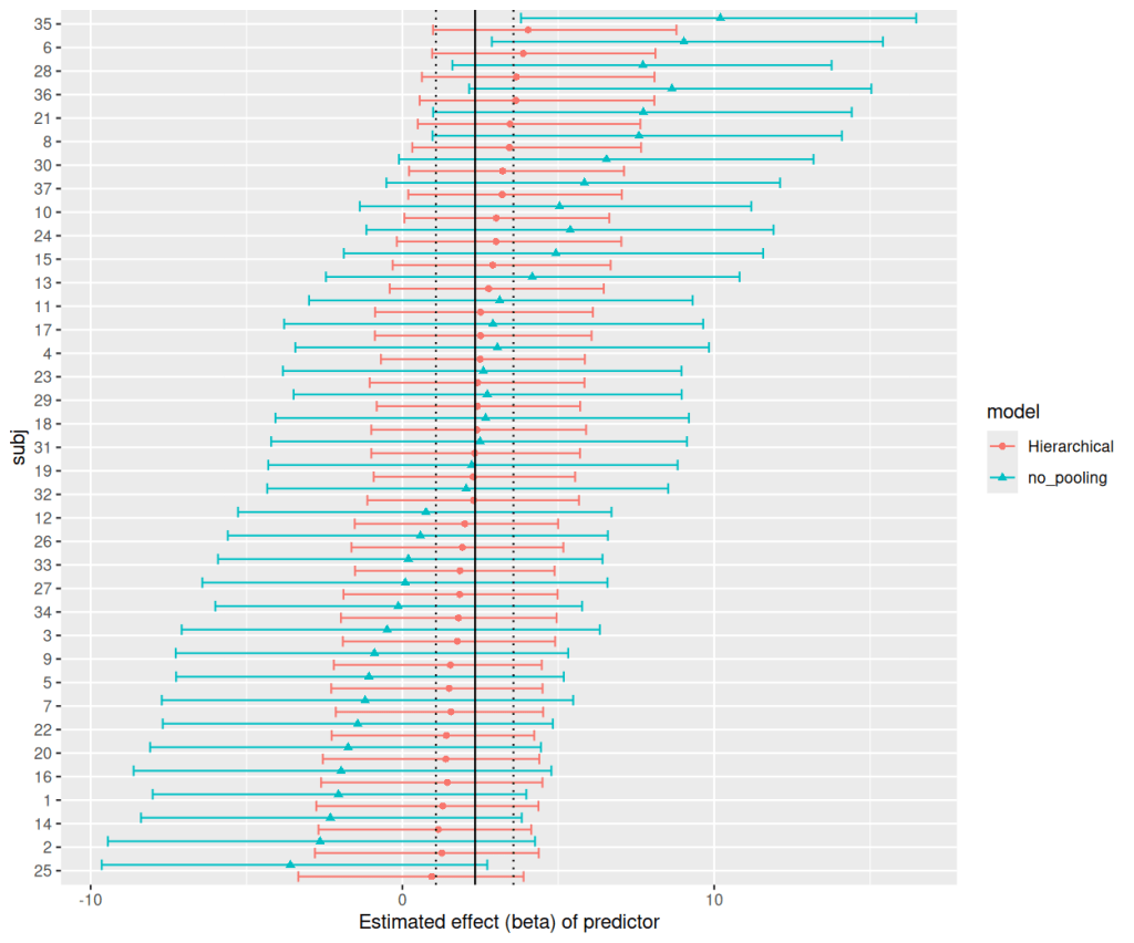
As briefly introduced earlier, when we model data using a normal distribution in the likelihood function, each observation is seen as a random sample from a normal distribution that represents a specific group within the hierarchical model. In this context, the mean and the mean effects of regulators (independent variables) in each group are treated as random samples from shared distributions across all groups. In other words, each group deviates (varying effect) from the grand mean (referred to as alpha or Intercept, which is a fixed effect) and from the grand mean effects of regulators (betas, which are also fixed effects). Hence, hierarchical models are also called mixed effects models. And they shrink the group-level variations towards the grand means, generating smaller deviations compared to results from no-pooling models. The group-level deviations are defined by taus (SD in brms), while the individual-level variation is represented by sigma.

###############################
### data with one predictor ###
###############################
## read in data
data_h

## centralize data
data_h=data_h %>% 
  mutate(c_predictor=predictor-mean(predictor))

# histgram plot of data overlay with density of normal distribution
ggplot(data=data_h)+
  geom_histogram(aes(x=output,y=after_stat(density)),
                 binwidth=5,
                 color="grey",
                 alpha=0.5)+
  #plot stat function for density of normal distribution, extracting mean and sd of original data
  stat_function(fun=dnorm,
                args=list(mean=mean(data_h$output),
                          sd=sd(data_h$output)))
#~~~~~~~~~~~~~~~~~~~~~~#
#~# complete pooling #~#
#~~~~~~~~~~~~~~~~~~~~~~#
data_h_cp=brm(output~1+c_predictor,
              data=data_h, family=gaussian(),
              prior=c(prior(normal(0,50),class=Intercept),
                      prior(normal(0,10),class=b,coef=c_predictor),
                      prior(normal(0,50),class=sigma)))

data_h_cp
plot(data_h_cp)

#~~~~~~~~~~~~~~~~~~~~~~#
## no pooling ##
#~~~~~~~~~~~~~~~~~~~~~~#
data_h_np=brm(output~0+factor(subj)+c_predictor:factor(subj), #note,do not write 0+1:factor(subj)+c_predictor:factor(subj), 1:factor(subj) will not fit an intercept for each group!
              data=data_h,family=gaussian(),
              # the following essentially set the same priors for all intercepts and slops
              prior=c(prior(normal(0,50),class=b),
                      prior(normal(0,50),class=sigma)))
data_h_np
data_h_np %>% posterior_summary()

data_h_np %>% 
  as_draws_df() %>%  #this returns as tibble, as.data.frame() returns a data frame, the formats are the same. column as variable, row as samples
  select(ends_with("c_predictor")) %>% 
  rowMeans()

data_h_np %>% 
  as.data.frame() %>% 
  select(ends_with("c_predictor"))

#~~~~~~~~~~~~~~~~~~~~~~#
## hierarchical model without intercept-slop correlation ##
#~~~~~~~~~~~~~~~~~~~~~~#
data_h_h=brm(output~1+c_predictor+(1+c_predictor||subj), # the same as c_predictor+(c_predictor||subj)
             data=data_h,
             family=gaussian(),
             prior=c(prior(normal(0,50),class=Intercept),
                     prior(normal(0,10),class=b,coef=c_predictor),
                     prior(normal(0,50),class=sigma),
                     prior(normal(0,10),class=sd,coef=Intercept,group=subj),
                     prior(normal(0,10),class=sd,coef=c_predictor,group=subj)))

data_h_h
variables(data_h_h)
# plot with mcmc_dense on selected variables
#   the top 5 parameters are your posteriors
#   the rest are group level adjustments
mcmc_dens(data_h_h,pars=variables(data_h_h)[1:5])

# extract group level adjustments on c_predictor and plot
#   construct the names, which is also the column names you want to extract
groupAdjNames=paste0("r_subj[",1:37,",c_predictor]")
groupAdjNames

# #   posterior sampling and extraction (as.data.frame(modelResult) or as_tibble(modelResult))
# groupAdjsamples=as.data.frame(data_h_h) %>% 
#   select(all_of(groupAdjNames))
# #   calculate the mean
# groupAdjsamples_mean=colMeans(groupAdjsamples)

#   getting posterior summary directly for above adjustments to slope
#   by default output data.frame with row names, correspond and ranked by subj
groupAdjsSum=posterior_summary(data_h_h,variable = groupAdjNames) %>% 
  # change to tibble to remove row-names
  as_tibble() %>% 
  # add subj column (factor at the end to keep the order)
  mutate(subj=1:n()) %>% 
  # rank by mean
  arrange(Estimate) %>% 
  # factor subj to keep the order
  mutate(subj=factor(subj,levels=subj))
  
groupAdjsSum

#   plot
ggplot(groupAdjsSum, aes(x=Estimate,xmin=Q2.5,xmax=Q97.5,y=subj))+
  geom_point()+
  geom_errorbar()+
  xlab("Group-level adjustments to effect of predictor")

## compare the effect with no pooling method
#   the complication is in no pooling model, the output is direct effect from predictor
#   whereas in hierachical model, the output is adjustment and you need to add them to ground beta
# extract data_h_np effects of c_predictor estimated for each subject
np_sub_effect=posterior_summary(data_h_np,variable=paste0("b_factorsubj",unique(data_h$subj),":c_predictor")) %>% 
  as_tibble() %>% 
  mutate(subj=1:n(),
         model="no_pooling")
np_sub_effect

# extract hierarchical model, posterior sampling of the grand mean of beta#
#   make sure all samplings are in vector (n=4000)
h_beta=c(as_draws_df(data_h_h)$b_c_predictor)
h_beta
# extract adjustments from each subj, these are also sampling, 4000x37variables, each column is for a subj
#   use as_draws_matrix other than as_draws_df to remove hidden reserved variable such as .chain, .iteration, and .draw
#   however use as_draws_matrix will contains meta data "draw", it looks like a column, but it is not
h_beta_adj=as_draws_matrix(data_h_h,variable=groupAdjNames)
h_beta_adj
# add mean with adjustments, then use as.data.frame to remove metadata "draw",
#   the vector of h_bet will be added to each column
h_beta_sub=as.data.frame(h_beta+h_beta_adj)
# calculate mean, 95% credible intervals for each column
#   lapply will apply function to each column, the function output will be a tibble with one row
#     the tibble column name correspond to np_sub_effect
#     this will generate a list of one-raw-tibbles
# bind_row of this list of tibbles will generate one tibble
h_sub_effect=lapply(h_beta_sub,function(x){
  tibble(Estimate=mean(x),
         Q2.5=quantile(x,0.025),
         Q97.5=quantile(x,0.975))
}) %>% 
  bind_rows() %>% 
  mutate(model="Hierarchical",
         subj=1:n())
h_sub_effect

# bind betas of no-pooling and hierarchical model together
np_h_sub_effect=bind_rows(np_sub_effect, h_sub_effect) %>% 
  arrange(Estimate) %>% 
  # factor after arrange, will group same subj (of two models) into one factor level
  mutate(subj=factor(subj,levels=unique(.data$subj)))
np_h_sub_effect

# plot
# getting grand mean and CI of beta
h_b_effect=posterior_summary(data_h_h,variable="b_c_predictor")
h_b_effect

# plot with flipped position first, because position_dodge() (not overlapping the tow lines) can only do horizontal shift of the two types of model, while keeping them still in one column
ggplot(np_h_sub_effect, aes(x=subj,ymin=Q2.5,ymax=Q97.5,y=Estimate,color=model,shape=model))+
  geom_point(position=position_dodge(1))+
  geom_errorbar(position=position_dodge(1))+
  #add the mean and 95% CI for hierarchical model
  geom_hline(yintercept=h_b_effect[,"Estimate"])+
  geom_hline(yintercept=h_b_effect[,"Q2.5"],linetype="dotted")+
  geom_hline(yintercept=h_b_effect[,"Q97.5"],linetype="dotted")+
  coord_flip()+
ylab("Estimated effect (beta) of predictor")

Hierarchical model with correlated varying intercept and slope

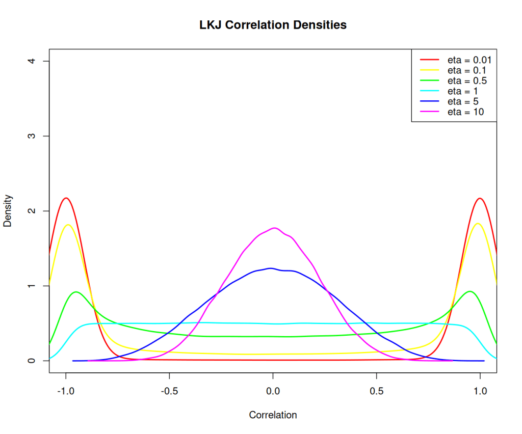
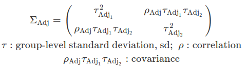
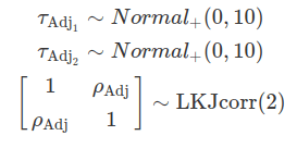
In some cases, it is reasonable to assume that the group-level variation regarding the grand mean and the variation concerning the mean effect of a regulator are correlated. These correlations are defined by a variance-covariance matrix and are assumed to follow a multivariate normal distribution. The likelihood function remains unchanged compared to an uncorrelated scenario; however, the differences arise from the choice of priors. These correlations are often modelled using LKJ priors.

The Lewandowski-Kurowicka-Joe distribution (LKJ) is a high-dimensional probability distribution for a d x d positive definite matrix with a unit diagonal. It has a single shape parameter, eta, taking values in the range(0, infinity). When eta equals to one, the distribution is uniform across the parameter space, making it uninformative and assigning equal probabilities to all ranges of correlation values. As eta increases from one, the probability distribution peaks at zero correlations; whereas when eta decreases from one, the distribution favours extreme correlation values. Setting ETA equal to two is often considered a relatively uninformative choice for variables that exhibit a small degree of correlation.

One caution is that the between-group variance can not be modelled here. Although we can obtain adjustments on the grand beta from each level of a group, we can not conclude about the differences this regulator has on these groups.

############################
### explore LKJ function ###
############################
# stan-dev/cmdstanr
# devtools::install_github("stan-dev/cmdstanr")
# rmcelreath/rethinking
# devtools::install_github("rmcelreath/rethinking")
library(cmdstanr)
library(rethinking)

scan_eta=c(0.01,0.1,0.5,1,5,10)
n_dim=2  # dimension of correlation matrix
n_samples=100000
plot(NULL, xlim=c(-1, 1), ylim=c(0, 4), xlab="Correlation", ylab="Density", main="LKJ Correlation Densities")
colors <- rainbow(length(scan_eta))
for (i in seq_along(scan_eta)) {
  samples <- rlkjcorr(n = n_samples, K = 2, eta = scan_eta[i])
  dens <- density(samples[,1,2])
  lines(dens, col=colors[i], lwd=2)
}
legend("topright", legend=paste("eta =", scan_eta), col=colors, lwd=2)

#~~~~~~~~~~~~~~~~~~~~~~#
## hierarchical model with correlation ##
#~~~~~~~~~~~~~~~~~~~~~~#
data_h_h_cor=brm(output~1+c_predictor+(1+c_predictor|subj), # the same as c_predictor+(c_predictor|subj)
             data=data_h,
             family=gaussian(),
             prior=c(prior(normal(0,50),class=Intercept),
                     prior(normal(0,10),class=b,coef=c_predictor),
#sigma models within group variation
                     prior(normal(0,50),class=sigma),
# sd models group-level standard deviation (tau)                     prior(normal(0,10),class=sd,coef=Intercept,group=subj),
                     prior(normal(0,10),class=sd,coef=c_predictor,group=subj),
                     #use lkj to define correlation between sd_Intercept and sd_c_predictor
                     prior(lkj(2),class=cor,group=subj)))

# the model output too many variables
variables(data_h_h_cor)
# only plot the top 6
plot(data_h_h_cor,nvariables=6)

Maximal hierarchical model

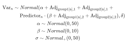
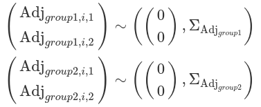
We can also use multiple variables to group observations, such as subjects and experimental measurements. Additionally, we assume correlations between each group variable’s variation to the intercept and slope. This is called the ‘maximal’ hierarchical model. At this stage, we consider the estimates for one grouping variable to be independent from others. Therefore, we define how each group variable independently adjusts the intercept (alpha) and slope (beta).

#~~~~~~~~~~~~~~~~~~~~~~#
## hierarchical model with two grouping variables and correlations between adjustment for intercept and slope for each group ##
##  so called maximal model ##
#~~~~~~~~~~~~~~~~~~~~~~#
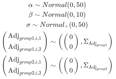
priors_full=c(prior(normal(0,50),class=Intercept),
              prior(normal(0,10),class=b,coef=c_predictor),
              prior(normal(0,50),class=sigma),
              
              ## para for group: subj
              prior(normal(0,10),class=sd,coef=Intercept,group=subj),
              prior(normal(0,10),class=sd,coef=c_predictor,group=subj),
              #use lkj to define correlation between sd_Intercept and sd_c_predictor
              prior(lkj(2),class=cor,group=subj),
              
              ## para for group: item
              prior(normal(0,10),class=sd,coef=Intercept,group=item),
              prior(normal(0,10),class=sd,coef=c_predictor,group=item),
              #use lkj to define correlation between sd_Intercept and sd_c_predictor
              prior(lkj(2),class=cor,group=item))

# you can also simply priors, use one sd for all coef and all groups; and one cor
priors_simple=c(prior(normal(0,50),class=Intercept),
              prior(normal(0,10),class=b,coef=c_predictor), # you can ignore coef=c_predictor here as well
              prior(normal(0,50),class=sigma),
              prior(normal(0,10),class=sd), # ignore coef and group means this will be for all coefs and all groups
              prior(lkj(2),class=cor) #ignore group means this will be for all groups
              )

data_h_h_cor=brm(output~1+c_predictor+(1+c_predictor|subj)+(1+c_predictor|item), # the same as c_predictor+(c_predictor|subj)+(c_predictor|item)
                 data=data_h,
                 family=gaussian(),
                 prior=priors_simple)

variables(data_h_h_cor)
plot(data_h_h_cor,nvariables=4)

## posterior check on #
pp_check(data_h_h_cor,ndraws=40, type="dens_overlay")
pp_check(data_h_h_cor,ndraws=100,type="dens_overlay_grouped",group = "subj")+
  # put legend (about y and y_rep) inside the graph other than on the side
  theme(legend.position = "inside",
        legend.position.inside = c(.5,.08))
# try to print within group sd, so see whether model capture within group diversity
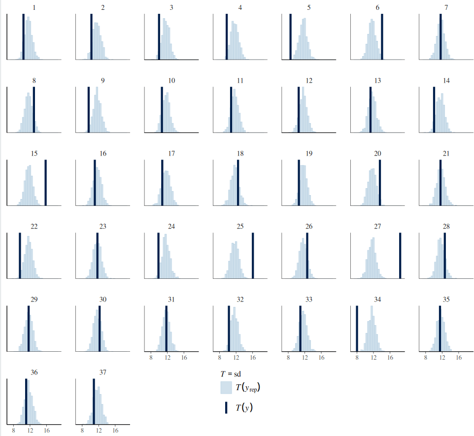
pp_check(data_h_h_cor,ndraws=1000,type="stat_grouped",group="subj",stat="sd",
         facet_args=list(scales="fixed"))+
  scale_x_continuous(breaks=c(8,12,16),limits=c(7,19))+
  theme(legend.position = "inside",
        legend.position.inside = c(.5,.08))

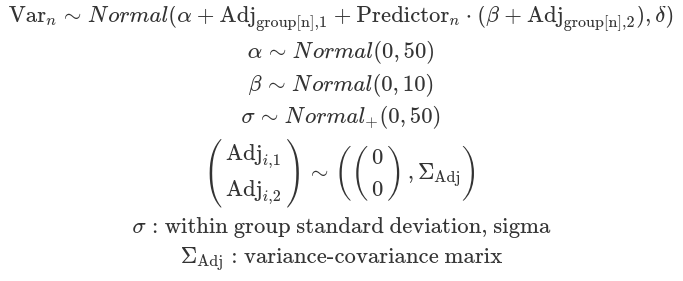
Distributional regression model

Most of the Bayesian hierarchical models, as shown above, primarily focus on adjusting the location (mu), which includes parameters like alpha, beta, as well as the adjustments made at each group level and the correlations between these adjustments. However, the scale parameter (sigma) is typically treated as a constant across all groups and individuals. This assumption can lead to misfitting models that fail to accurately capture noise at each group level, resulting in the estimated SD diverging from the observed SD for each cluster of data. This assumption is often considered a default and tends to be overlooked by researchers (for further discussion see https://cran.r-project.org/web/packages/brms/vignettes/brms_distreg.html).

Such a misfit can be rectified by defining deviations for sigma for each group (variation for within-group variation). In this context, the within-group sigma is treated as a random sample drawn from a single distribution of sigmas, which has a fixed grand mean, and group-level variations. This is called a distributional model. Typically, we exponentiate the formula of sigma (so sigma is modelled on the log scale) to ensure that any negative deviations from the ‘location’ do not result in negative numbers. The brm function models sigma (as well as sd) class parameters in the log scale, and it exponentiates them while sampling. This is to ensure these parameters remain positive. Although users do not need to transform these posterior distributions, their prior distributions should be defined on the log scale.

#~~~~~~~~~~~~~~~~~~~~~~#
## hierarchical model with 
#   two grouping variables and 
#   correlations between adjustment for intercept and slope for each group 
#   model within group variation on sigma ##
#~~~~~~~~~~~~~~~~~~~~~~#
# brms will automatically model sigma in log scale.
#   this means the priors for sigma need to be on defined on log scale
# no need to exp the posterior
priors_sigma=c(prior(normal(0,50),class=Intercept),
               prior(normal(0,10),class=b,coef=c_predictor), # you can ignore coef=c_predictor here as well

               prior(normal(0,10),class=sd), # ignore coef and group means this will be for all coefs and all groups
               prior(lkj(2),class=cor), #ignore group means this will be for all groups
               
               #define intercept and sd for sigma
               prior(normal(0,log(40)),class=Intercept,dpar=sigma),
               prior(normal(0,5),class=sd,group=subj,dpar=sigma))

data_h_h_cor_sd=brm(
  brmsformula(output~1+c_predictor+(1+c_predictor|subj)+(1+c_predictor|item),
              #define between group variance
              sigma~1+(1|subj)),
  prior=priors_sigma,
  data=data_h
)

variables(data_h_h_cor_sd)
#use variable= to define who to plot out
posterior_summary(data_h_h_cor_sd)
plot(data_h_h_cor_sd,variable=c("b_sigma_Intercept","sd_subj__sigma_Intercept"))

# look at the sigma
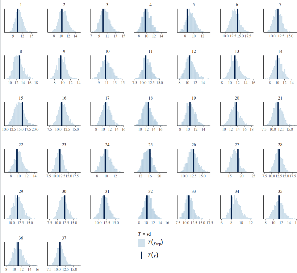
pp_check(data_h_h_cor_sd,type="stat_grouped",ndraws=1000,stat="sd",group="subj")+
  theme(legend.position = "inside",
        legend.position.inside = c(.5,.08))

The complexity and structure of a Bayesian hierarchical model depend on several factors, including domain knowledge, the parameter of interest, the number of observations (as more complex models require more data within each group and more groups), and available computing power. There are no straightforward rules to follow. For instance, if we anticipate greater variance at the group level compared to within-group variance, it is beneficial to allow for group-level adjustments on sigma. However, this adjustment is not necessary for all group variables; in other words, it is not essential to apply a maximal hierarchy to sigma in every case.

Log-normal for likelihood function

We can also apply a log-normal distribution as the likelihood function. This distribution is particularly well-suited for modelling response times to stimuli, as it effectively represents positive continuous variables (for more information, see our blog post on the log-normal distribution). It’s important to note that the parameters, including alpha, beta, sigma, and tau (sd), are defined on the log scale for both priors and posteriors. The exception to this is ETA, which is used to define the correlations between group-level adjustments for intercept and slope in LKJ priors. ETA should not be logged.

Sometimes, it is necessary to use contrast coding for effector values. Effector values are often imbalanced across different factor levels (e.g. -1 for one-third of the observations and +1 for the others). Unlike previous models where effector values are centralised (post here), in this case, the alpha represents the value of the dependent variable when the effector value is zero (e.g. no effector value or without experimental manipulation), rather than corresponding to the grand mean of effector values. Hence, the prior for alpha should have an adjusted “location” aligning with this interpretation.

After fitting the model, it is often advisable to sample from prior distributions of some parameters and compare these samples with their corresponding posterior samples. If a large discrepancy exists between prior and posterior distributions for a particular parameter, it is recommended to conduct a prior sensitivity analysis.

In a prior sensitivity analysis, a series of prior distributions for the parameter should be fitted through the model. The mean and the 95% confidence interval of the corresponding posteriors should then be reported. If the parameter of interest is beta, it is important to demonstrate how the posterior differs in response to changes in the effector value. In practice, this illustrates how the dependent variable changes in response to a step-wise change in the effector value, using the sampled posterior beta. When using a log-normal as the likelihood function, the median difference to effector-value change is a better choice than the mean. Because the median of a log-normal distribution is influenced only by the mu of the log-transformed normal distribution (exp(mu)), whereas the mean is affected by both mu and sigma (exp(mu+sigma^2/2)) (see this post). Finally, we can report the mean of the posterior median difference between effector values, taking into account the sampling of different parameters, such as alpha and beta.

After prior sensitivity analysis, the posterior we report back should be the one associated with multiple priors. A robust posterior distribution should remain unaffected by changes in its priors. As a rule of thumb, prior distributions should not be overly strong or too specific (narrow). Instead, using a less informative and relatively broader prior will allow the data to have a greater influence on the posterior, which is our goal. It is important to include posteriors derived from informative priors based on previous research, and from sceptical priors reflecting the opinions of scientific opponents, in addition to the uninformative prior identified during the sensitivity analysis.

#########################################################
### Hierarchical model with log-normal for likelihood ###
#########################################################
## read in data
data("df_stroop")
df_stroop
data_lognormal=df_stroop %>% 
  mutate(cond=if_else(condition=="Incongruent",1,-1)) %>% 
  mutate(result=RT) %>% 
  select(subj,cond,result)

data_lognormal
## fit the model
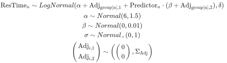
fit_lognormal=brm(result~cond+(cond|subj),
                  family=lognormal(),
                  data=data_lognormal,
                  prior=c(prior(normal(6,1.5),class=Intercept),
                          prior(normal(0,0.01),class=b,coef=cond),
                          prior(normal(0,1),class=sigma),
                          prior(normal(0,1),class=sd),
                          prior(lkj(2),class=cor,group=subj)))


# check beta 
posterior_summary(fit_lognormal,variable="b_cond")

### comparie posterior and prior sampling on beta and see distance ###
b_posterior_samples=as_draws_df(fit_lognormal)$b_cond
b_posterior_samples
b_prior_samples=rnorm(mean=0,sd=0.01,n=length(b_posterior_samples))
b_prior_samples

b_samples=tibble(samples=c(b_posterior_samples,b_prior_samples),
                 distribution=c(rep("posterior",length(b_posterior_samples)),
                         rep("prior",length(b_prior_samples))))           

ggplot(b_samples,aes(x=samples,color=distribution))+
  geom_density(alpha=0.5)+
  ggtitle("Prior and Posterior comparisons of beta")


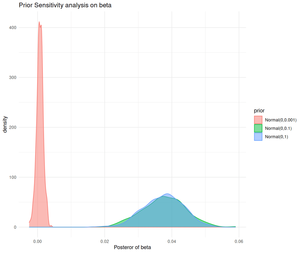
### prior sensitivity analysis
## set up a prior_list for beta 
# scan only three as example and save time
beta_prior_list=list("Normal(0,0.001)"=prior(normal(0,0.001),class=b,coef=cond),
                     # "Normal(0,0.01)"=prior(normal(0,0.01),class=b,coef=cond),
                     # "Normal(0,0.05)"=prior(normal(0,0.05),class=b,coef=cond),
                     "Normal(0,0.1)"=prior(normal(0,0.1),class=b,coef=cond),
                     # "Normal(0,0.5)"=prior(normal(0,0.5),class=b,coef=cond),
                     "Normal(0,1)"=prior(normal(0,1),class=b,coef=cond)
                     # "Normal(0,2)"=prior(normal(0,2),class=b,coef=cond)
                     )

## the other priors
other_priors=c(prior(normal(6,1.5),class=Intercept),
               prior(normal(0,1),class=sigma),
               prior(normal(0,1),class=sd),
               prior(lkj(2),class=cor,group=subj))

## set up the fitting result
beta_fit_list=list()

## go though the prior list then append the fit list
for(priorname in names(beta_prior_list)){
 #first combine the priors
 full_priors=c(other_priors,beta_prior_list[[priorname]])
 # fit the model
 fit=brm(result~cond+(cond|subj),
      family=lognormal(),
      data=data_lognormal,
      prior=full_priors,
      #reduce the chain and iter here for speed
      iter=500,chains=2,silent=TRUE,
      # the following is important for calculating Bayes Factor
      save_pars = save_pars(all = TRUE))
 # append the result
 beta_fit_list[[priorname]]=fit
}

## gather posterior summary
posterior_summary_result=tibble()
for(priorname in names(beta_prior_list)){
  posterior_summary_result=rbind(posterior_summary_result,posterior_summary(beta_fit_list[[priorname]],variable="b_cond"))
}
posterior_summary_result

## plot density for each model
posterior_sample=map_dfr(names(beta_fit_list),function(pname){
  as_draws_df(beta_fit_list[[pname]]) %>% 
    select(b_cond) %>% 
    mutate(prior=pname)
})
posterior_sample

ggplot(posterior_sample,aes(x=b_cond,fill=prior,color=prior))+
  geom_density(alpha=0.5)+
  labs(title="Prior Sensitivity analysis on beta",x="Posteror of beta",y="density")+
  theme_minimal()

### calculate LOO (leave one out) ###
# iterate through data points to leave one data point out at each time, before fitting, then used fitted model to predict that data point
# elpd_diff = difference in expected log pointwise predictive density (ELPD) between each model and the best model (the one with the highest ELPD).
#   Higher ELPD → better out-of-sample prediction.
#   elpd_diff = 0 for the top model.
#   Negative values = worse predictive performance.
# se_diff: uncertainty in that difference
# Large diff + small SE	Strong evidence of real difference
LOO_result=lapply(beta_fit_list,loo)
LOO_result
loo_compare(LOO_result)

### Bayese Factor calculation ###
#   BF is ratio of marginallikelihood 
#   marginal likelihood can be considered as an average of the likelihood across the entire prior.
#   therefore BF is very much dependent on priors
#   
library(bridgesampling) #for calculating marginal likelihood
bridge_result=lapply(beta_fit_list,bridge_sampler)
bridge_result
bf(bridge_result[["Normal(0,0.1)"]],bridge_result[["Normal(0,0.001)"]])
bf(bridge_result[["Normal(0,0.1)"]],bridge_result[["Normal(0,1)"]])
bf(bridge_result[["Normal(0,1)"]],bridge_result[["Normal(0,0.001)"]])