Regression tells us how the dependent (the output) variable responds to changes in independent variables that can be categorical, ordinal or continuous.
In following sections, I show how three linear models can be defined by Bayesian statistics while the dependent variable follows different likelihood functions. Although the formulae are linear, the relationship between dependent and independent variables may not be linear.
Normal Distribution for likelihood function
We have a set of measurements of the size of an object. We hypothesize that it is influenced by a quantifiable predictor. We assume that the relationship is linear, however, we know little about the object and the predictor.
We model the size as normally distributed, although this is not strictly correct as it can not be zero or negative. Based on our hypothesis, the mean of the normal distribution (the average size), alpha, is linearly influenced by the predictor whose effect is determined by beta. There are noises or variabilities in the measuring process determined by sigma and it is also normally distributed.

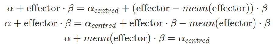
In the following model, we centre predictor values, by subtracting the mean from every value (hence “c” in the name). Therefore, the intercept, object size seemingly unaffected by the predictor, is assessed at the average predictor value (0 in the centralized case). If the predictor is not centralised, the intercept is evaluated at zero effector size.
Due to the lack of prior information about the size and how it can be affected by the predictor, we chose a set of uninformative priors. We assumed small, bidirectional effects (reduction or increase) from the predictor.
packs=c("brms","rstan","bayesplot","dplyr","purrr","tidyr","ggplot2","ggpubr","extraDistr","sn","hypr","lme4","rootSolve","bcogsci","tictoc")
lapply(packs, require, character.only = TRUE)

select = dplyr::select
extract = rstan::extract

# read in data

# centralize the effector
testdata=testdata %>%
  mutate(c_effector=effector-mean(effector))

fit_normal_result=brm(
  # define the linear relationship:
  #   1 represents intercept alpha which is not affected by effector
  #   even if omit 1, brms will still fit for intercept
  #   if really want to remove intercept, then use 0+ or -1+
  # c_effector will be multiplied by beta;
  #   using centralized effector so the intercept reflects value at mean effector size
  size~1+c_effector,
  data=testdata,
  family=gaussian(),
  # set prior for Intercept, alpha: uninformative between 0-2000
  prior=c(prior(normal(1000,500),class=Intercept),
          #set prior for sigma, brms will automatically truncate it to be more than zero
          # uninformative prior between 0-2000
          prior(normal(0,1000),class=sigma),
          #set prior for beta, and indicate it is the beta for c_effector: uninformative -200 - 200
          #set the same prior for different effectors, omit coef
          prior(normal(0,100),class=b,coef=c_effector))
)

fit_normal_result

plot(fit_normal_result)
By default, brms centres all predictors before sampling to increase efficiency. Therefore, brms assumes the prior and posterior distribution of the intercept at the mean effector size. If predictors are not centred by users, there will be a discrepancy between the brms output and the user expectation. As shown below, the difference in the intercept between none-centred and centred predictor is the mean multiplied by beta. However, when the mean or the beta is extremely small or when the prior for the intercept is very wide, this discrepancy is trivial.
We can explicitly instruct brms to fit the intercept for none-centred predictors as follows.
### use none-centred predictor ###
# note the linear relationship and prior class
fit_normal_nonecentre_result=brm(
  # define the linear relationship:
  #   0 indicates removal of effector-centred intercept
  #   Intercept is reserved word, here for none-effector-centred intercept
  size~0+Intercept+effector,
  data=testdata,
  family=gaussian(),
  # set prior for Intercept, alpha: this prior shifted to left compare with prior used above.
  #   as this is the intercept with zero effector value
  # note, the class here is not Intercept, but b
  prior=c(prior(normal(800,200),class=b,coef=Intercept),
          #set prior for sigma, brms will automatically truncate it to be more than zero
          prior(normal(0,1000),class=sigma),
          prior(normal(0,100),class=b,coef=effector))
)
To interpret model results, we can use mean and two standard deviations to calculate the 95% confidence interval for the beta of the predictor. We can also calculate the percentage of randomly drawn positive values from the posterior distribution to assess how likely the effect is positive.
Finally, we check how well this model represents the data by overlaying posterior predictive distributions with observed data for each representative predictor value (first graph below). we also look at summary stats such as mean size distribution for each predictor value comparing with the mean value from real data (second graph below).


## get posterior predictive distribution density for every effector value 0:5
#   then overlay with the real observation
# However, pp_check can not group effector (or c_effector) as it is a continuse variable, unless you change it to categorical prior to model fitting
#   so the following will just flashing the 6 effector value so far not plotting them together
for(i in 0:5){
  # generate sub data from observation
  subdata=filter(testdata,effector==i)
  # use pp_check to generate posterior prediction for effector
  p=pp_check(fit_normal_result,
             type="dens_overlay",
             ndraws=100,
             newdata=subdata)+
    geom_point(data=subdata,aes(x=effector,y=0.00001))
  print(p)
}

# use bayesplot and group by effector value
yrep <- posterior_predict(fit_normal_result, ndraws = 1000)
y <- testdata$size
ppc_violin_grouped(y, yrep,  group= testdata$effector, probs = c(.1,.9), alpha = 0.1, y_draw = "points", y_size = 1.5)
ppc_dens_overlay_grouped(y, yrep,  group= testdata$effector)

# use bayesplot to overlay mean between prediction and real value
ppc_stat_grouped(y,yrep,group=testdata$effector,stat="mean")
Log-normal distribution for likelihood function
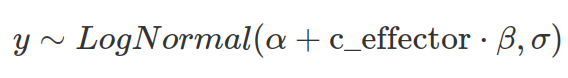
The log-normal distribution is often used to model the positive continuous variable with a long tail. To define a log-normal distribution, the mean and standard deviation of the log-transformed data (under normal distribution) are used. Therefore, when the log-normal distribution is used as the likelihood function, prior and posterior distributions are log-transformed. When using log-normal distribution to model the linear relationship between the dependent and independent variables, the linearity is defined between the mean of log-transformed data and independent variables. As a result, the actual effects from independent variables are multiplicative and grow exponentially (see the blog post on the log-normal distribution).
To define prior distributions for the location and scale of a log-normal distribution, one can log-transform the parameters specifying the prior for the mean of the none-log-transformed distribution (as a guess for the log-transformed normal distribution). However, it is not intuitive to set up priors for sigma and beta. It is better to draw prior predictive distributions to assess how these parameters interact and to calibrate sigma and beta.
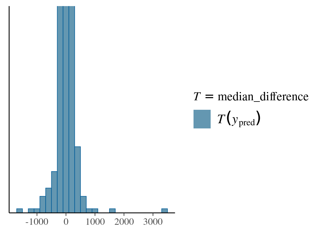
In the following example, we use the prior predictive distribution to calibrate beta and find its value range that gives reasonable response differences between adjacent effector values.
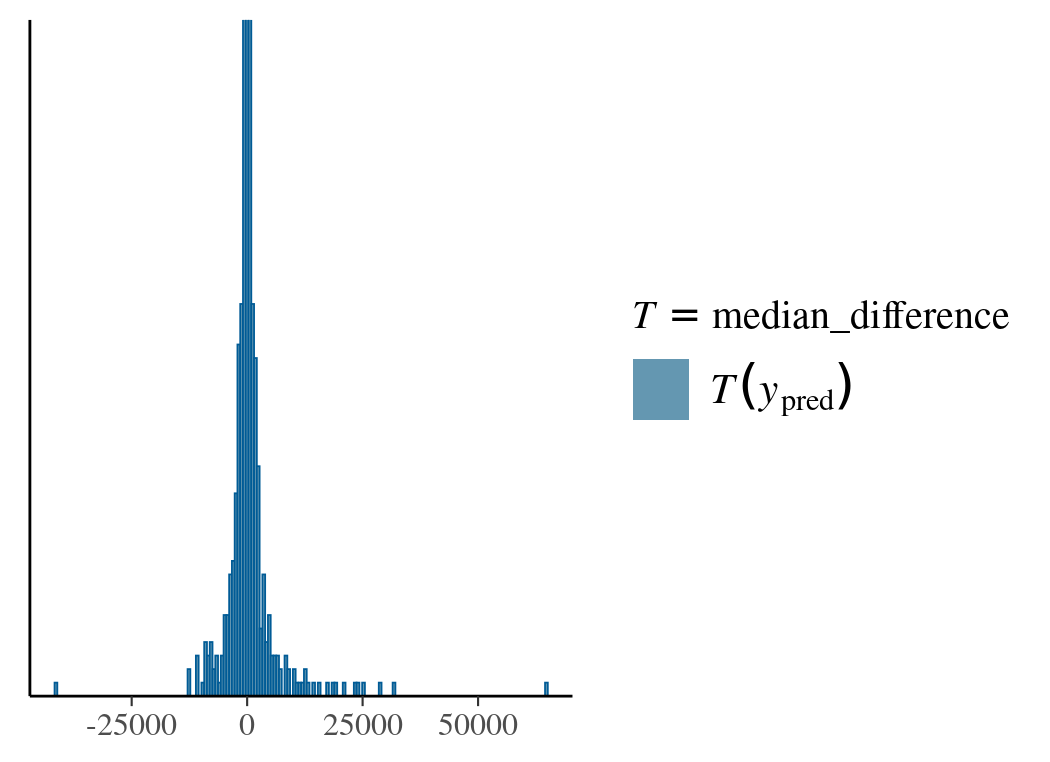
After sampling from priors, we provide the pp_check function with a custom function to calculate the median response differences. The reason for using the median other than the mean is due to the mean’s dependence on both beta and sigma. In the first prior choice (Normal(0,1)) for beta, the predicted value for the dependent variable is widely spread with extreme values. The second choice (Normal(0,0.01)) is more reasonable.
# read in data

# centre the effector
testdata2=testdata2 %>%
  mutate(c_effector=effector-mean(effector))
testdata2

### prior predictive distribution
## run brm model fitting without real data and sample_prior only
# set up ref data
testdata2_ref=testdata2 %>%
  mutate(time_ms=rep(1,n()))

testdata2_ref

# fit model for prior only
fit_prior_sample=brm(time_ms~1+c_effector,
                     data=testdata2_ref,
                     family=lognormal(),
                    prior=c(prior(normal(6,1.5),class=Intercept),
        prior(normal(0,1),class=sigma),
#prior(normal(0,1),class=b,coef=c_effector)
# a smaller spread of beta
prior(normal(0,0.01),class=b,coef=c_effector)
                             ),
                     sample_prior = "only",
                     control = list(adapt_delta = .9))

# prior predictive check with pp_check
# define function for median difference
#   lag(x) is to find the previous value; lead() would be find next value
median_difference=function(x){
  median(x-lag(x),na.rm=TRUE)
}

pp_check(fit_prior_sample,
         type="stat",
         stat="median_difference",
         prefix="ppd", #prior predictive distribution
         binwidth=200
         )+coord_cartesian(ylim=c(0,50))
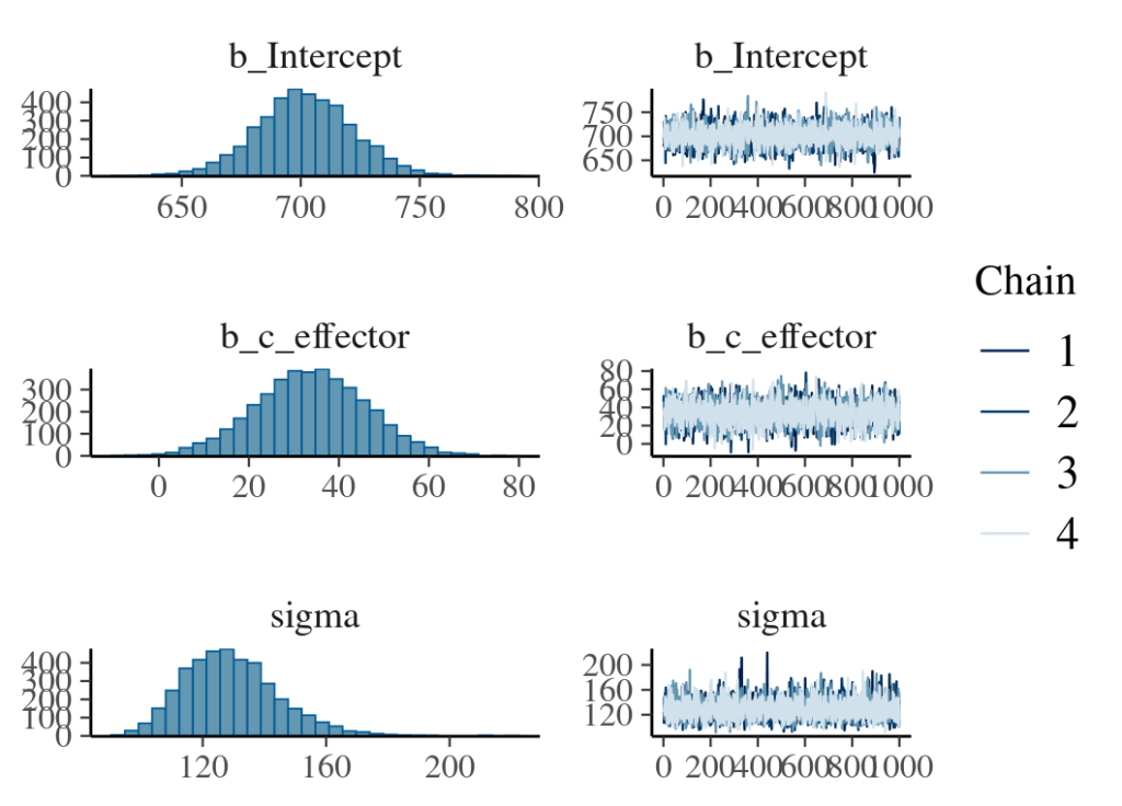
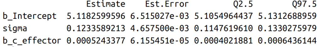
After fitting the model, the first step of communicating results is to make a posterior summary of model parameters (means and confidence intervals ) and plot them (see figures below). An obvious focus here is to assess the effect of the influencer: beta. As units for all posterior parameters are log-transformed, it is better to change them back by the exp() function.

In a log-normal model, the influencer’s effect is not linearly added to the mean of the dependent variable. In other words, the same change in the independent variable do not result in the same alteration in the dependent variable. Rather, the dependent variable changes exponentially depending on the current value of the independent variable. The following formula shows that the step-wise increases in the effector size, assuming each increase is 1, brings varying differences, depending on the constant alpha, beta and the variable that is the exponentially transformed current effector size.
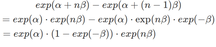
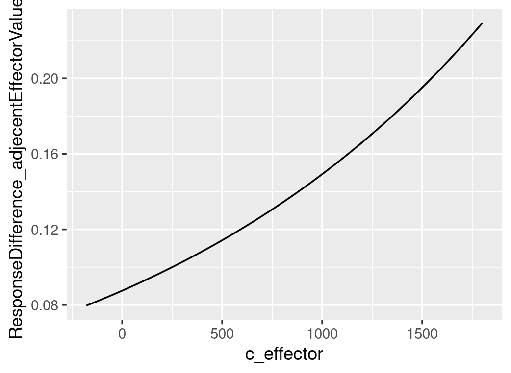
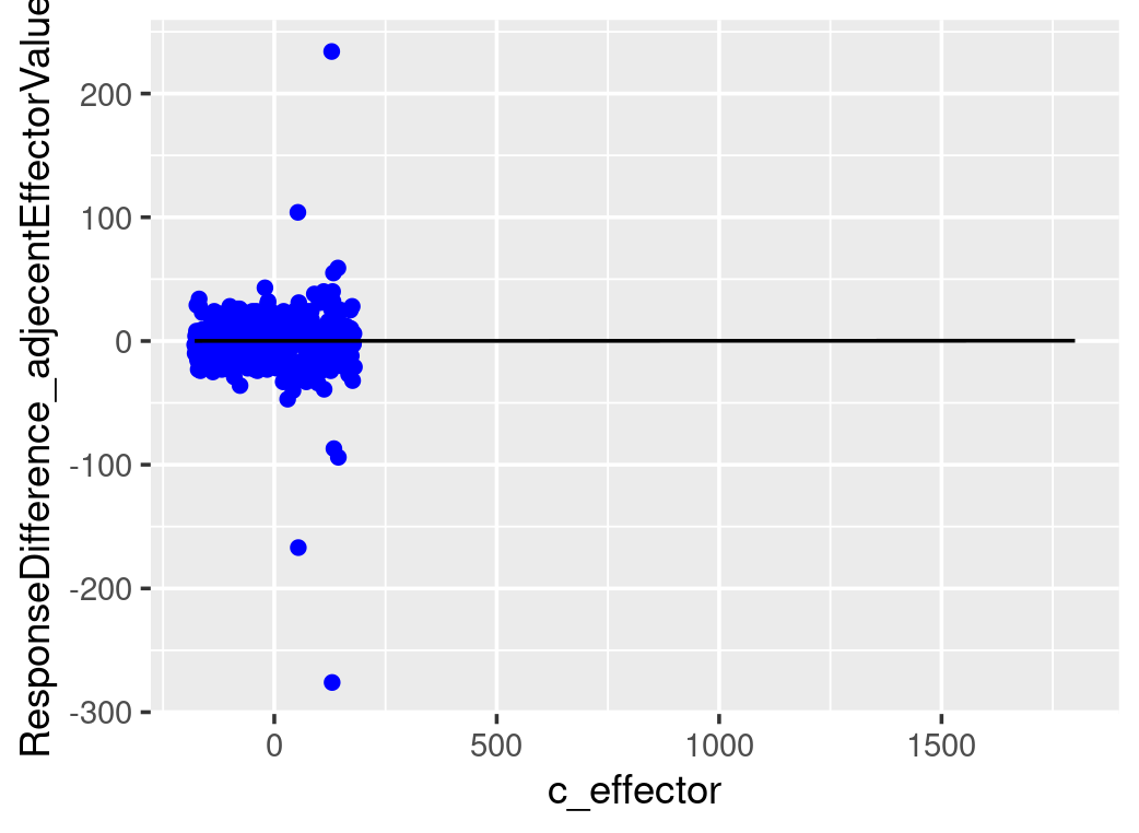
The plots below show that the step-wise differences in the dependent variable, in response to a constant increase in the effector size, rise exponentially. However, as the beta is minimal, both predicted and real step-wise differences show almost flat growth in the range of effector size available in the data. The value of the parameter beta is minimal. However, it remains positive across the 95% confidence interval. To prove how significant is this effective size, we will need to calculate the Bayes Factor.
#~~~~~~~~~~~~~~~~~~~~~~~~~~~~~~~~~~~#
### fitting the model ###
#~~~~~~~~~~~~~~~~~~~~~~~~~~~~~~~~~~~#
# fit brms model with real data
fit_lognormal_result=brm(time_ms~1+c_effector,
                         family=lognormal(),
                         data=testdata2,
                         prior=c(prior(normal(6,1.5),class=Intercept),
                                 prior(normal(0,1),class=sigma),
                                 prior(normal(0,0.01),class=b,coef=c_effector))
                         )


# quick check model fitting and result
plot(fit_lognormal_result)

# use posteior_summary for specific variable.
#   all variables except sigma are produced with "b_" as prefix.
posterior_summary(fit_lognormal_result,
                  variable=c("b_Intercept","sigma","b_c_effector")
                  )

#~~~~~~~~~~~~~~~~~~~~~~~~~~~~~~~~~~~#
###       communicate results     ###
#~~~~~~~~~~~~~~~~~~~~~~~~~~~~~~~~~~~#
## demonstrate the multiplicative effect from effector
# draw posterior samples, draw means (Intercept), draw beta (b_c_effector)
as_tibble(fit_lognormal_result)

# alpha_draws=as_tibble(fit_lognormal_result)$b_Intercept
# although it seems as_tibble(fitresult) can retrieve random draws from posterior sample, as_draws_df is a better choice
alpha_draws=as_draws_df(fit_lognormal_result)$b_Intercept
beta_draws=as_draws_df(fit_lognormal_result)$b_c_effector

# calculate the differences in dependent variable value
#   between mean-effector-value (as effector is centered, this will result in the intercept value)
#     and one-step-size-ahead-effector-value (here we assume one step size is 1)
differences_middle=exp(alpha_draws)-exp(alpha_draws-1*beta_draws)
mean(differences_middle)
quantile(differences_middle,c(0.025,0.975))

## calculate the mean difference (among all the alpha and beta) between all effector values and its 1-step-ahead values
# due to small beta value, use higher effector value to show the differences are growing exponentially
testdata2
min(testdata2$c_effector)
max(testdata2$c_effector)

#shift_c_effector=seq(min(testdata2$c_effector)+1,max(testdata2$c_effector),by=1)
shift_c_effector=seq(min(testdata2$c_effector)+1,1800,by=1)
# use map2_dfr from purrr to calculate differences between all effector values and its previous-step-values, as row
#   therefore, each row correspond to one alpha and one beta value
differences=map2_dfr(alpha_draws,beta_draws,
                     function(a,b){
                       tibble(t(tibble(value=(exp(a+shift_c_effector*b)-exp(a+(shift_c_effector-1)*b)))))
                     })
# calculate column mean/median, that is mean difference of each effector value and one-step-ahead value pair, calculated based on all alpha and beta
dim(as.matrix(differences))
mean_differences=colMeans(as.matrix(differences))
median_differences=apply(as.matrix(differences),2,median)
mean_differences
median_differences

stepWiseDifferences=tibble(c_effector=shift_c_effector,
                           mean_difference=mean_differences,
                           median_difference=median_differences)

stepWiseDifferences
filter(stepWiseDifferences,c_effector==0) #check if this value correspond to the one calculated above

# get the difference from the testdata2
testdata2_stepWiseDiff=(testdata2$time_ms-lag(testdata2$time_ms))[2:length(testdata2$time_ms)]
testdata2_stepWiseDiff=tibble(c_effector=shift_c_effector,stepWiseDiff=testdata2_stepWiseDiff)

# plot all the differences, use c_effector as x and mean_difference as y
ggplot()+
  geom_point(data=testdata2_stepWiseDiff,aes(x=c_effector,y=stepWiseDiff),color="blue")+
  geom_line(data=stepWiseDifferences,aes(x=c_effector,y=mean_difference))+
  ylab("ResponseDifference_adjecentEffectorValues")
So far, we have focused on how the influencer affects the mean of log-transformed data. By exponential transformation, we have obtained the median of the log-normal distribution. To get the mean of the log-normal distribution, we must factor in the sigma (exp(.+sigma^2/2) please see the blog post on log-normal distribution to understand the conversions of these parameters between these two distributions). Alternatively, we can use the built-in function fitted() to calculate the mean effects. To use this function, a new data frame is needed, which contains all effector values we want to get posterior samples on (these need to be in one column with the same column name as in the original data used to fit the model). The result is a matrix with each effector value corresponding to a column, and posterior samples to rows. The function fitted() is different from posterior_predict(). Function fitted() gives the expected values of the dependent variable based on the random draws from posterior distributions of parameters; whereas posterior_predict() randomly samples the dependent variable from the likelihood function based on posterior distributions of parameters.
#~~~~~~~~~~~~~~~~~~~~~~~~~~~~~~~~~~~~#
### use fitted() to do posterior prediction ###
#~~~~~~~~~~~~~~~~~~~~~~~~~~~~~~~~~~~~#
# set up newdata frame containing all effect values you want posterior predictions on
newdata1=tibble(c_effector=seq(-180,1800,by=1))

# the prediction below is also based on sigma, not just alpha and beta, therefore we are looking at median change
predict1=fitted(fit_lognormal_result,
       newdata=newdata1,
       #to predict on newdata, you must turn summary off
       summary=FALSE)

predict1[1,]
dim(predict1)[2]

#pair-wise column wide calculation of differences
# method 1 (for loop): the following is very slow
difference_matrix=tibble(tibble(predict1[,2])-tibble(predict1[,1]))
dim(difference_matrix)
for(n in 3:dim(predict1)[2]){
  newcol=tibble(tibble(predict1[,n])-tibble(predict1[,n-1]))
  difference_matrix=bind_cols(difference_matrix,newcol)
}

# method 2 (across and lag)
difference_matrix=predict1 %>% t %>% as.data.frame %>%
  mutate(across(everything(),~.-lag(.))) %>% t %>% as.data.frame %>%
  select(-c(1))

# BEST: method 3 (two shifted matrixes and calculate difference in one go)
difference_matrix=predict1[,2:dim(predict1)[2]]-predict1[,1:(dim(predict1)[2]-1)]

# BEST: method 4 (use diff)
difference_matrix=t(diff(t(predict1)))

# calculate colMean
dim(difference_matrix)
difference_matrix_mean=colMeans(difference_matrix)
difference_matrix_mean
dim(difference_matrix_mean)

tibble(c_effector=seq(-179,1800,by=1),
       difference=difference_matrix_mean) %>%
  ggplot()+
  geom_line(aes(x=c_effector,y=difference))

#~~~~~~~~~~~~~~~~~~~~~~~~~~~~~~~~~~~~~~~~~~~#
### use posterior_predict () do the above ###
#~~~~~~~~~~~~~~~~~~~~~~~~~~~~~~~~~~~~~~~~~~~#
# posterior_predict() is different from fitted () gives expected values based on draws of posterior parameter (the dependent variable is not random draw);
#   whereas posterior_predict() gives random draws (the dependent variable) from the likelihood function that is based on the random draws of posterior parameter
predict2=posterior_predict(fit_lognormal_result,
                           newdata=newdata1)
dim(predict2)

# use the following across and lag(), however, it only works on rows of a data frame, so we need to transpose twice
difference_matrix2=predict2 %>% t %>% as.data.frame %>%
  mutate(across(everything(),~.-lag(.))) %>% t %>% as.data.frame() %>%
  #remove the first column
  select(-c(1))
dim(difference_matrix2)

difference_matrix2_mean=colMeans(matrix(difference_matrix2))
difference_matrix2_mean

tibble(c_effector=seq(-179,1800,by=1),
       difference=difference_matrix2_mean) %>%
  ggplot()+
  geom_line(aes(x=c_effector,y=difference))
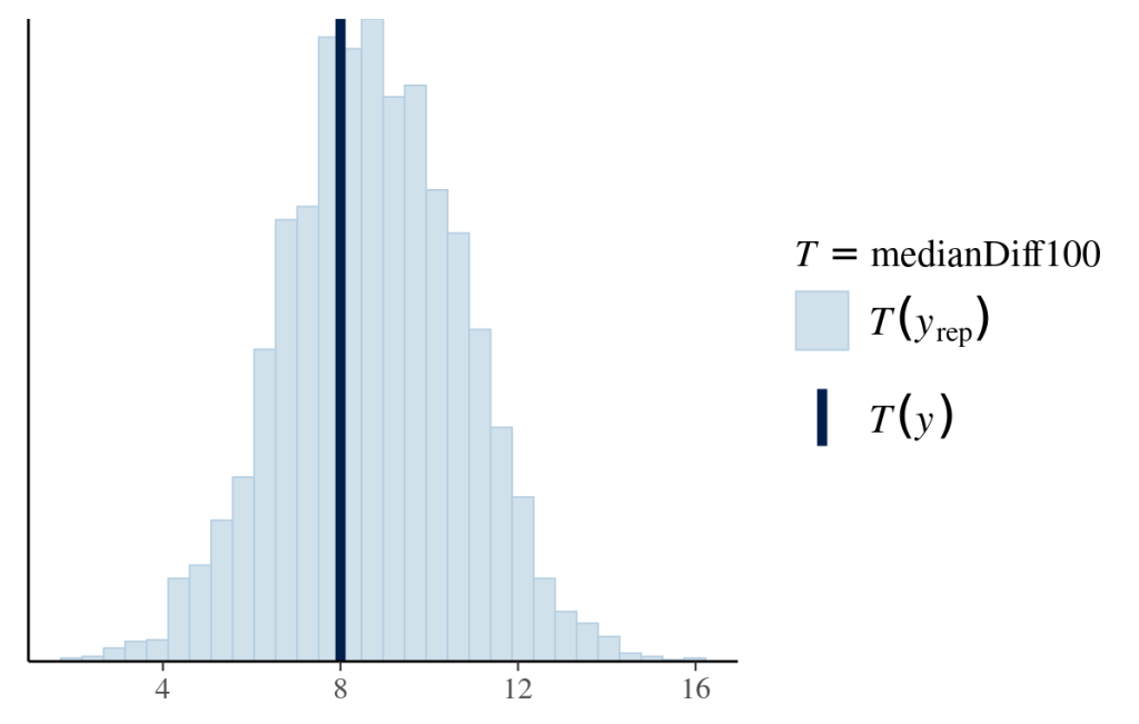
As it only shows a noticeable difference in response to a 100-increase in the effector value, we will compare the distribution of median differences for every 100-increase between the posterior predictions and data. Each median difference in the dependent variable is calculated from one likelihood function based on one set of posterior parameters. The distribution of medians is constructed by all the posterior samples. The following graph shows that the model-predicted median differences match the observed median difference.
#~~~~~~~~~~~~~~~~~~~~~~~~~~#
### descriptive adequacy ###
#~~~~~~~~~~~~~~~~~~~~~~~~~~#
# define function to calculate median 100-increase difference in response
medianDiff100=function(x){
  # lag(x,n) obtains the value of nth previous value
  # if there is no 100th previous value, then it returns NA
  # therefore for calculating median, you need to remove NA
  median(x-lag(x,100),na.rm=TRUE)
}
# put this function in pp_check()
pp_check(fit_lognormal_result,
         type="stat",
         stat="medianDiff100")
Logistic Regression
Imagine a dependent variable that can only be zero or one with an unknown probability of getting one, like Bernoulli trails. We want to know how an independent variable affects this probability. A linear regression model that results in unbounded real values is improper to model the probability because a probability is between zero and one.
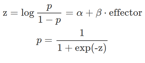
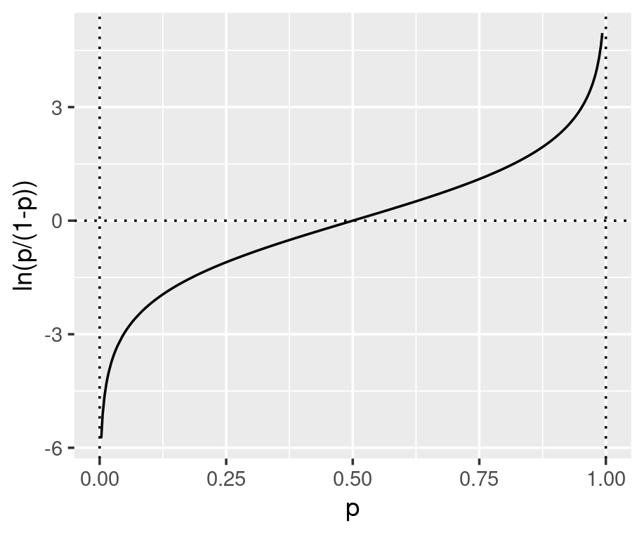
Under the generalised linear model (GLM) framework, a link function is defined to connect the output from the linear regression to the quantity we want to estimate. One GLM is logistic regression which uses the log-odds as the link function and directly connects the linear regression to the value of the log-odds (see equation below). As shown in the graphs below, the log-odds convert a probability value between 0 and 1, to a real number between negative and positive infinity.
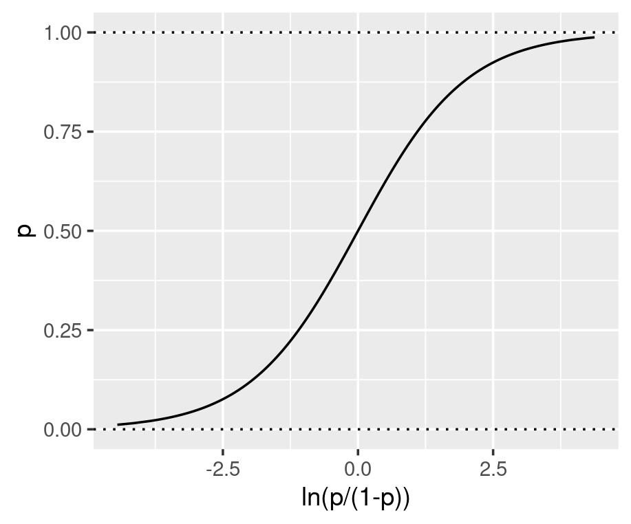
The parameters inside the linear equation are not directly related to the probability, but the log-odds. The relationship between the probability and the output from linear regression is not linear or logarithmic, but logistic. Function qlogis(prob) and plogis(log-odds) can convert probability and log-odds.
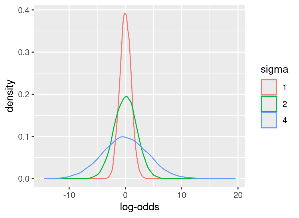
As parameters are on the log-odds scale, their priors are defined on the log-odds scale as well. Therefore, conversions from the log-odds to probability are necessary to make sense of these prior distributions. Most importantly, prior predictive checks can indicate how these parameters interact. For instance, alpha in the above equation represents the log-odds at the mean-effector value. We can assume the mean-effector value results in a probability centred around 0.5 with much uncertainty. From function qlogis(0.5), we know the log-odds of 0.5 is 0. We can define a normal distribution at the mean of zero for alpha. However, it is tricky to estimate how big the sigma is or how uncertain the alpha is, as some choices can result in meaningless probability values. The following graphs show different prior distributions for alpha and their corresponding probability density. Some priors emphasize extreme probabilities and sigma at 1 is a better choice.

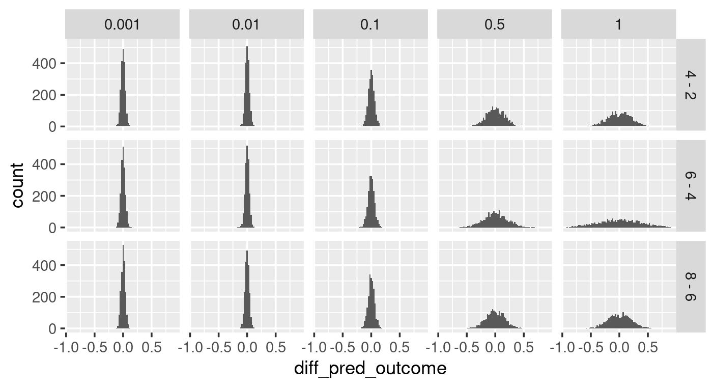
When choosing the prior for beta, we can assume that the effector most likely does not influence the outcome by setting up a normal distribution centred around 0. We can explore the uncertainty around beta by prior predictive checking with various sigma values. As shown in the left graph below (sigma as x, and effector values as y for the facet grid), some sigma values for beta’s prior distribution give high probabilities to extreme outcomes (e.g. sigma of 1). The differences in the outcome caused by the incremental growth of effector value (right graph below), show that some choices of sigma give possibilities to bigger differences in outcome that may not be realistic. With all these in mind, a sigma of 0.1 is a good choice for beta.

##############################################################
#### logistic function as a linker between probability and linear regression ####
##############################################################
# logistic regression explanatory plot
# show how probability is converted to real number without boundary
p=runif(5000,min=0.0001,max=0.999)
# z=log(p/(1-p))
z=qlogis(p) #use default location,0, and scale,1 will replicate log(p/(1-p))

ggplot(data=tibble(p=p,z=z))+
  geom_line(aes(x=p,y=z))+
  ylab("ln(p/(1-p))")+
  geom_hline(yintercept=0,linetype=3)+
  geom_vline(xintercept=c(0,1),linetype=3)

# show how to convert link to p
z=rnorm(50000,mean=0,sd=1)
#p=1/(1+exp(-z))
p=plogis(z) # use default location,0, and scale,1, will replicate results of p=1/(1+exp(-z)) this is not simply formula 1/(1+exp(-z))

ggplot(data=tibble(z=z,p=p))+
  geom_line(aes(x=z,y=p))+
  xlab("ln(p/(1-p))")+
  geom_hline(yintercept=c(0,1),linetype=3)

#~~~~~~~~~~~~~~~~~~~~~~~~~~~~~~~~~~~~~~~~~~~~~~~~~~~~~~~~~~~~~~~~~~~~~~~~~~~~~~~~~~~~~~~~~~~~~~~~~~~~~~~~~~~#
### explore log-odds' priors defined by normal distribution and their corresponding probability densities ###
#~~~~~~~~~~~~~~~~~~~~~~~~~~~~~~~~~~~~~~~~~~~~~~~~~~~~~~~~~~~~~~~~~~~~~~~~~~~~~~~~~~~~~~~~~~~~~~~~~~~~~~~~~~~#
alphas=bind_rows(tibble(`log-odds`=rnorm(10000,mean=0,sd=4),sigma=4),
                 tibble(`log-odds`=rnorm(10000,mean=0,sd=2),sigma=2),
                 tibble(`log-odds`=rnorm(10000,mean=0,sd=1),sigma=1)) %>%
  mutate(sigma=factor(sigma))
probs=bind_rows(tibble(prob=plogis(rnorm(10000,mean=0,sd=4)),sigma=4),
                tibble(prob=plogis(rnorm(10000,mean=0,sd=2)),sigma=2),
                tibble(prob=plogis(rnorm(10000,mean=0,sd=1)),sigma=1)) %>%
  mutate(sigma=factor(sigma))

ggplot(alphas)+
  geom_density(aes(x=`log-odds`,colour = sigma))

ggplot(probs)+
  geom_density(aes(x=prob,colour=sigma))

#~~~~~~~~~~~~~~~~~~~~~~~~~~~~~~~~~~~~~~~~~~~~~~~~~~~#
#### prior predictive check with custom function ####
#~~~~~~~~~~~~~~~~~~~~~~~~~~~~~~~~~~~~~~~~~~~~~~~~~~~#
# use map2_dfr from purrr to put iterate through a pair of parameters, alpha and beta into a function.
#   also need to rotate effector value here, here effector_values is an array containing repeats, the repeats is sample_size/realNo_unique_effector_value
# procedures:
#   putting each alpha, beta pair into the linear equation with centralized c_effector_values
#   change the outputs from the linear equation (log-odds) to probabilities by plogis(log-odds) function
#   then use the probabilities to randomly retrieve bernoulli trials.

prior_predict_check_func=function(alphas,betas,effector_values,
                             sample_size){
  map2_dfr(alphas,betas,function(alpha,beta){
    tibble(effector_values=effector_values,
           #center effector_values
           c_effector_values=effector_values-mean(effector_values),
           # c_effector_values is an array of values
           probs=plogis(alpha+c_effector_values*beta),
           # use rbern from extraDistr package for randomly sampling from bernoulli distribution
           # here probs is an array of probs calculated for each c_effector_values.
           #  the returned prediction will be of sample_size, not sample_size x probs_number
           #    therefore the sample_size is evenly spread for each prob
           prior_pred=rbern(sample_size,prob=probs))
    #every iter is a different set of alpha-beta
    }, .id="iter") %>%
    # convert iter from str to number
    mutate(iter=as.numeric(iter))
}

testprob=c(0.1,1)
testprob=rep(c(0.1,1),20)
testprob
length(rbern(40,prob=testprob))
rbern(40,prob=testprob)

##  getting alphas (log-odds), betas(log-odds), and effector_values (not centered)
# retrieve alphas from its prior (the normal distribution) (remember alpha is log-odds, 0 is actually represent a probability of 0.5)
alphas=rnorm(2000, mean=0,sd=1)

# retrieve betas, the prior for beta is normal distribution centered around 0 (assuming effector has no effect)
#   however, several sigmas worth a try.
beta_sigmas=c(1, 0.5, 0.1, 0.01, 0.001)

# effector values, repeat each of them to the sample size you want for each, then the total correspond to the sample_size for above function
effector_values=rep(c(2,4,6,8),300)
sample_size=1200

# use map_dfr to iterate through beta's sigma, and within this function call for the prior_predict_check_func
# this function will pile all the data frames together
# you will get a data-frame with this amount of rows 5(beta_sd)*2000*1200(samples) or 5(beta_sd)*2000*4(effector values)*300(sample for each effector)
prior_pred_check=map_dfr(beta_sigmas,function(sd){
  betas=rnorm(2000,mean=0,sd=sd)
  prior_predict_check_func(alphas, betas,effector_values,sample_size) %>%
    mutate(beta_sigma=sd)
})

prior_pred_check

## calculate average on each level, alpha-beta iter, beta_sd, effector_value
prior_pred_check_average=prior_pred_check %>%
  group_by(iter,effector_values,beta_sigma) %>%
  summarise(average_pred_output=mean(prior_pred),.groups="drop")

# levels: 1000(alpha-beta pairs)*5(beta_sd)*4(effector_values)
prior_pred_check_average

# facet_plot average_pred_output on beta_sigma and effector_values
ggplot(data=prior_pred_check_average)+
  geom_histogram(aes(x=average_pred_output),bins=50)+
  facet_grid(effector_values~beta_sigma)+
  scale_x_continuous(breaks = c(0,0.5,1))

## calculate lag average outcome based on adjacent effector values
prior_pred_check_average_diff=prior_pred_check_average %>%
  arrange(effector_values) %>%
  group_by(iter,beta_sigma) %>%
  mutate(diff_pred_outcome=average_pred_output-lag(average_pred_output)) %>%
  mutate(diff_effector_value=paste(effector_values,"-",lag(effector_values))) %>%
  filter(effector_values>2)

prior_pred_check_average_diff
unique(prior_pred_check_average_diff$diff_effector_value)

ggplot(prior_pred_check_average_diff)+
  geom_histogram(aes(diff_pred_outcome),bins=80)+
  facet_grid(diff_effector_value~beta_sigma)
The model fitting is straightforward setting the likelihood follows the Bernoulli distribution with a logistic linker. However, the posterior interpretations of model parameters are not intuitive as they are log-odds.
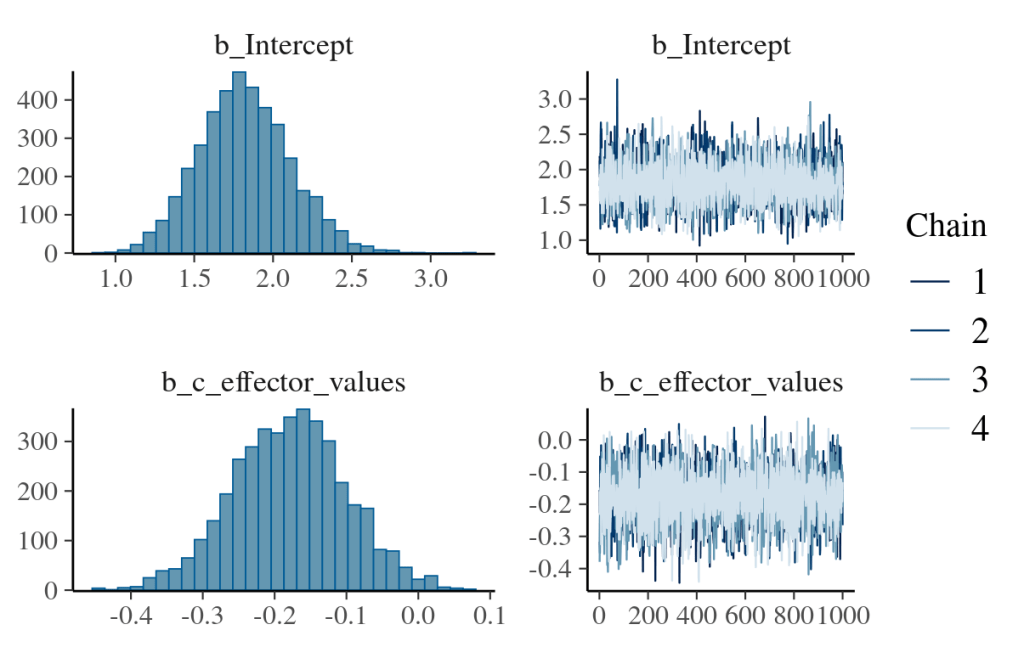
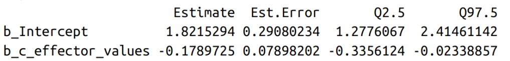
We can convert them back to probability by the plogis() function or the fitted() function. The latter is better as it can obtain the quantity of interest regardless of the linker function applied. As mentioned in the log-normal section, fitted() returns the converted linear-model result in the original data unit (exponential value for log-normal; probability between zero and one for log-odds). Although fitted() does samples from the posterior parameter spaces, it does not randomly sample from the likelihood function which is different from posterior_predict().
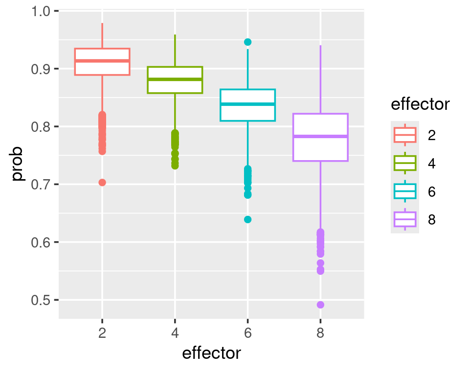
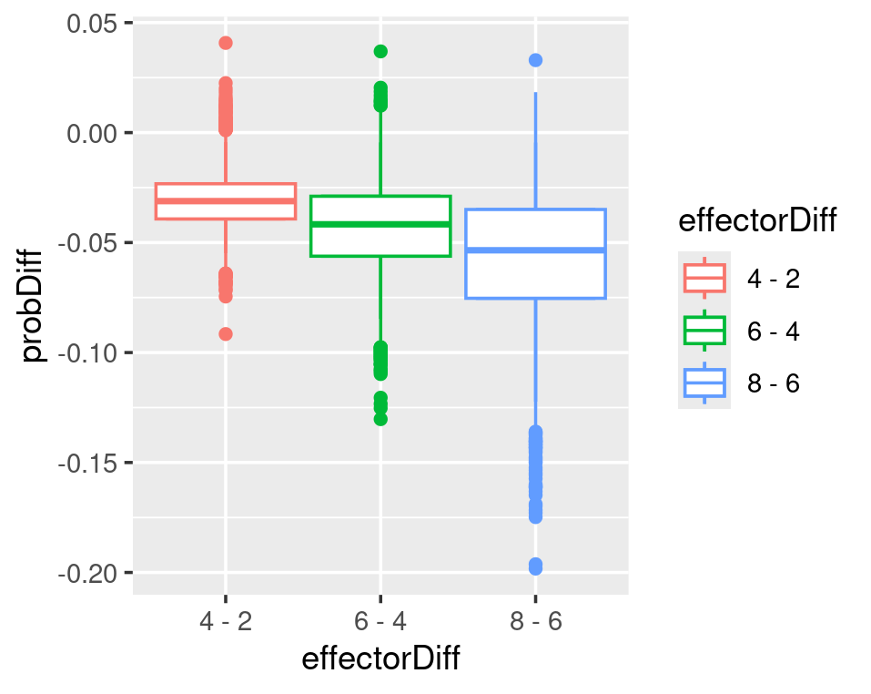
In a logistic regression model, the effector does not linearly affect the probability. Every unit increase of effector does not result in the same rise or decrease in probability. The plots below show that the biggest probability decrease occurs when the effector grows from 2 to 4. As the effector value increases, its effect on reducing the probability decreases.
#~~~~~~~~~~~~~~~~~~#
#### brms model ####
#~~~~~~~~~~~~~~~~~~#
## read in data, and centre the effector values
logisticRegression_data=logisticRegression_data %>%
  mutate(c_effector_values=effector_values-mean(effector_values))
logisticRegression_data

## model ##
# remember, for logistic regression we do not fit sigma, as we do not assume normal distribution for log-odds
logisticRegression_model_fit=brm(outcome~1+c_effector_values,
                                 data=logisticRegression_data,
                                 # define bernoulli trial
                                 family=bernoulli(link="logit"),
                                 prior = c(prior(normal(0,1),class=Intercept),
                                           prior(normal(0,0.1),class=b,coef=c_effector_values))
                                 )
## quick explore the results ##
# use posterior_summary for specific variable.
#   all variables are produced with "b_" as prefix.
posterior_summary(logisticRegression_model_fit,
                  variable=c("b_Intercept","b_c_effector_values")
)

plot(logisticRegression_model_fit)

#~~~~~~~~~~~~~~~~~~~~~~~~~~~~~~~~#
### Interpretation of log-odds ###
#~~~~~~~~~~~~~~~~~~~~~~~~~~~~~~~~#
## look at alpha, that is the outcome at average effector value (because we centered the effector before model fitting)
alpha_draws=as_draws_df(logisticRegression_model_fit)$b_Intercept
alpha_draws

# average outcome
c(mean=mean(plogis(alpha_draws)),quantile(plogis(alpha_draws),c(0.025,0.975)))

# use fitted(), first make effector values you are interested in into a new data
#   fitted() will sample from posterior parameter for alpha and beta
#   then return (if summary=FALSE, default) expected values from model fitting and results in data unit.
#   this is not random sampling from likelihood function.
#   if summay=TRUE, it will return the summary stats based on all values from all alphas and betas
newdata=data.frame(c_effector_values=0)
fitted(logisticRegression_model_fit,
       newdata=newdata,
       summary=TRUE)

## use fitted() to compute prob for each centred effector_values
effector_values=unique(logisticRegression_data$effector_values)
effector_values=effector_values[order(effector_values)]
c_effector_values=effector_values-mean(effector_values)
c_effector_values

newdata=data.frame(c_effector_values=c_effector_values)
newdata
fitted_p=fitted(logisticRegression_model_fit,
                newdata=newdata,
                summary=FALSE)
fitted_p
dim(fitted_p) #4000 rows (each corresponds to a pair of alpha and beta) 5 columns (each corresponds to one c_effector_values)

# use lag to compute difference between incremental increase of effector_values
#   lag can only compute row differences, other than colum difference, so I need to transpose, than use lag, then transpose back.
#   the first clumn will be NA
fitted_p_diff=t(t(fitted_p)-lag(t(fitted_p)))
# remove the first column
fitted_p_diff=fitted_p_diff[,2:dim(fitted_p_diff)[2]]
fitted_p_diff

#  calculate column mean
fitted_p_diff_mean=colMeans()
fitted_p_diff_mean

#~~~~~~~#
# plot the difference in prob with the effector_values differences
#~~~~~~~#
effector_values
effectorDiff=c()
for(i in 2:length(effector_values)){
  effectorDiff=append(effectorDiff,paste(effector_values[i],"-",effector_values[i-1]))
}
effectorDiff

plotdata=data.frame(effectorDiff=factor(effectorDiff),ProbDiff=fitted_p_diff_mean)
plotdata

# we can see that from 2 to 4 there is the biggest probability-difference and the differences are reducing when effector values increases
ggplot(plotdata)+
  geom_point(aes(x=effectorDiff,y=ProbDiff))

#~~~~~~~#
# re-plot above to have mean and quantiles in difference in prob
#~~~~~~~#
fitted_p_diff
plotdata=data.frame(fitted_p_diff) %>%
  setNames(effectorDiff) %>%
  pivot_longer(cols=everything(),names_to="effectorDiff",values_to = "probDiff") %>%
  mutate(effectorDiff=factor(effectorDiff))
plotdata

# define function to have 0.025 to 0.975 for ymin and ymax other than 25%-1.5IQR and 75%+1.5IQR
#   IQR being inter-quantile-range, which equals to the 75% quantile value in your data - 25% quantile value in your data
CI95=function(x) {
  r = quantile(x, probs = c(0.025,0.25,0.5,0.75,0.975))
  names(r) <- c("ymin", "lower", "middle", "upper", "ymax")
  return(r)
}

ggplot(plotdata,aes(x=effectorDiff,y=probDiff,color=effectorDiff))+
  geom_boxplot()+
  stat_summary(fun.data=CI95,geom="boxplot")

#~~~~~~~#
## the above plot might not be that obvious. How about we just plot the effector-value as x and all the probabilities calculated from pairs of alpha-beta in one graph?
#~~~~~~~#
fitted_p
effector_values
plotdata2=data.frame(fitted_p) %>%
  # tibble() %>%
  setNames(effector_values) %>%
  pivot_longer(cols=everything(),names_to = "effector",values_to = "prob")

plotdata2

ggplot(plotdata2,aes(x=effector,y=prob,color=effector))+
  geom_boxplot()+
  stat_summary(fun.data=CI95,geom="boxplot")
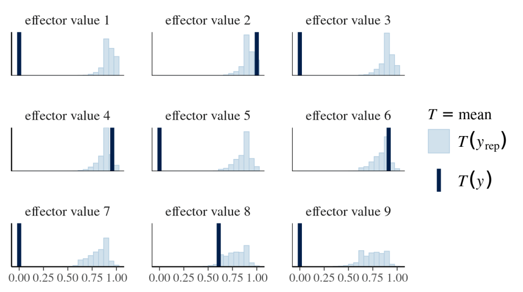
Finally, posterior predictive checks help not only align the prediction with existing data (effector values of 2,4,6 and 8) but also foresee the unknown (effector values of 1,3,5,7,9). The following graphs look at the distribution of mean outcomes based on samples derived from one effector value and all sampled alphas and betas.
#~~~~~~~~~~~~~~~~~~~~~~~~#
## posterior prediction ##
#~~~~~~~~~~~~~~~~~~~~~~~~#
# original exp data contains 4 effector values with 23 observations for each
logisticRegression_data %>%
  group_by(effector_values) %>%
  summarise(n=n())
# append the above data with effector value as 1,3,5,7,9, each of which have 23 observations with 0 as outcome
newdata=logisticRegression_data %>%
  bind_rows(tibble(effector_values=rep(c(1,3,5,7,9),23),
                   outcome=0,
                   # re-use the mean of original data to center the new effector value to be consistent with original Intercept interpretation
                   c_effector_values=effector_values-5))
newdata %>% group_by(effector_values) %>% summarise(n=n())
# set a list of names, whose name corresponds to centred effector values
effect_values_names = paste("effector value", 1:9) %>%
  setNames(-4:4)
effect_values_names

# use pp_check to do posterior prediction and plot.
#   pp_check will sample alphas and betas, then sample from each likelihood (bernoulli) based on each pair of alpha, beta, and effector value
#   the following asks to summarise the mean distribution for each effector value based on all sampled alphas and betas (thus all possible likelihood funcs)
#   and overlap with observed mean for each effector value
pp_check(logisticRegression_model_fit,
         newdata=newdata,
         type="stat_grouped",
         stat="mean",
         group="c_effector_values",
         bins=20,
         facet_args=list(ncol = 3, scales = "fixed",
                         labeller = as_labeller(effect_values_names)))
