For most Bayesian model fittings, there is no analytical solution for deriving posterior distributions or integrating them. Rather, we approximate those posteriors via random sampling from all possible parameter sets and their corresponding likelihood functions. Specifically, we sample posterior distributions from a multidimensional space, where each dimension corresponds to a parameter. The shape of this multifaceted space is determined by the priors and likelihood function.
Probabilistic programming languages, such as Stan, allow Bayesian inferences by reducing the complexity of sampling processes. The brms provides easy-to-use R functions for model fitting and sampling by using Stan at the back end.
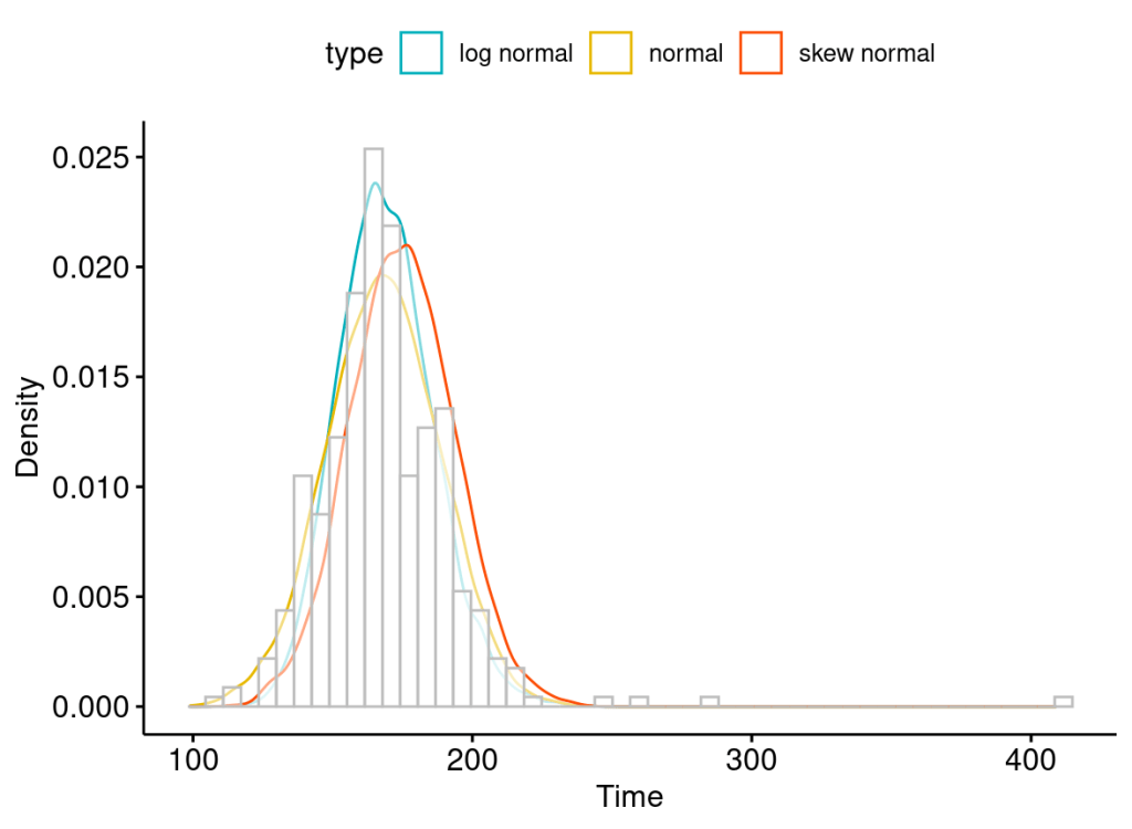
Let’s assume we have a skewed set of measurements about the time an individual spends on a task. We want to better understand the possibilities over time this individual needs.
packs=c("brms","rstan","bayesplot","dplyr","purrr","tidyr","ggplot2","ggpubr","#extraDistr","sn","hypr","lme4","rootSolve","bcogsci","tictoc")
lapply(packs, require, character.only = TRUE)

# read in your data
summary(testdata)
length(testdata$t)
sd(testdata$t)

normaldata=tibble(t=rnorm(10000,mean=168,sd=20),type="normal")
lnormaldata=tibble(t=rlnorm(10000,meanlog=5.124,sdlog=0.1),type="log normal")
skewnormaldata=tibble(t=rsn(10000,xi=168,omega=20,alpha=0.5),type="skew normal")

plotdata=bind_rows(normaldata,lnormaldata,skewnormaldata,tibble(t=testdata$t,type="data"))

# use ggpubr density for density plots, then add on geom object for histogram plot of data
ggdensity(data=filter(plotdata,type!="data"),x="t",
            #add="mean",
            rug=FALSE,
            palette = c("#00AFBB", "#E7B800", "#FC4E07"),
            color = "type",
            xlab="Time",ylab="Density")+ geom_histogram(data=testdata,aes(x=t),color="grey",fill="white",bins=50,alpha=0.5)
Likelihood Function
We can model the underlying distribution (likelihood function) of these measurements as a normal (symmetrical), a log-normal (right-skewed), or a skew–normal distribution (left or right-skewed).
By choosing a normal distribution for the likelihood function, we consider each measurement adds some variability/noise (![]() ) to a central true value (
) to a central true value ( ). The variability is normally distributed with a mean of 0 and a standard deviation of
  . This interpretation of a normal distribution gives us a simple linear equation with as the intercept (also as a dependent variable). The central value or intercept, , also called the location that lies on the mean of the normal distribution; indicates the scale that coincides with the standard deviation.


However, a more realistic distribution for modelling right-skewed (long right tail), none-negative (because the measurement is about time) data is a log-normal distribution. A Log-normal distribution is also defined by the locationand scalethat coincide with the mean and standard deviation of the log-transformed normal distribution. As they are on logged units of the original data, they are difficult to interpret. The location and scale derived from the log-normal distribution do not coincide with the mean and standard deviation of original data (unlogged) from the log-normal distribution.

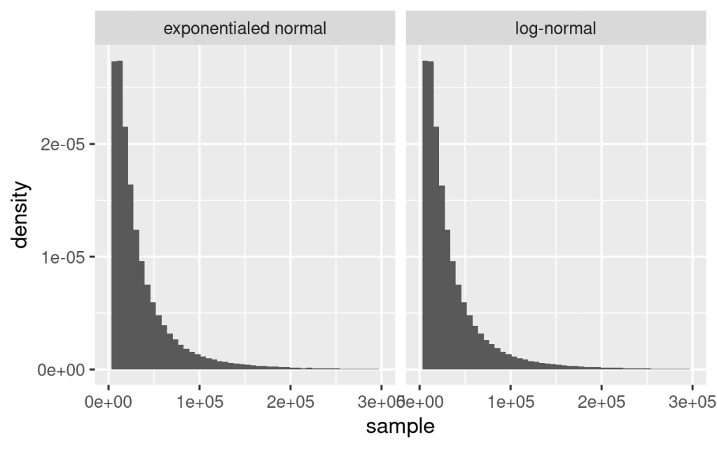
Based on the above equations, randomly sampled variables from a log-normal distribution, using and , assemble the same distribution derived from exponentially transformed variables sampled from a normal distribution, using the same and , as shown below.
############################
## LogNormal distribution ##
############################
mu=10
sd=1
N=1000000

# sln are samples following log-normal distribution, meaning these numbers, after being logged, follows normal distribution
#   sln~logNormal(mu,sd), so log(sln)~Normal(mu,sd)
# esn are exponentialed samples from normal distribution
#   esn~exp(Normal(mu,sd)), so log(esn)~Normal(mu,sd), therefore, esn~logNormal(mu,sd)
#   so esn follows the same distribution as sln
sln=rlnorm(N,meanlog=mu,sdlog=sd)
esn=exp(rnorm(N,mean=mu,sd=sd))

data2plot=bind_rows(tibble(sample=sln,type="log-normal"),
                    tibble(sample=esn,type="exponentialed normal"))

ggplot(data2plot,aes(sample))+
  geom_histogram(aes(y=after_stat(density)),bins=50)+
  facet_wrap(~type)+
  xlim(c(0,300000))
If a log-normal distribution is used as the likelihood function, the prior and posterior distributions are estimates of the location and scale which are the mean and standard deviation of the log-transformed data and having log-transformed units. Therefore, interpreting these parameters requires transforming sampled parameters by the exp() function. For the prior and posterior predictive distributions (here you are sampling predictions other than parameters), if drawn by custom functions, sampling from the log-normal distribution (rlnorm()) is recommended. If data was sampled from a normal distribution (rnorm()) instead, then use exp() function to transform them as you have essentially sampled from a log-transformed data set. If sampling these predictive distributions were achieved by one of the brms functions, the predictions assemble original data and have the same unit (e.g. posterior_predict(), pp_check()).
From the location and scale of the log-normal distribution (therefore from the mean and standard deviation of the log-transformed data in normal distribution), one can calculate the mean, median and standard deviation of the unlogged data (original data from the log-normal distribution) to better interpret the data on original unit.
The skew-normal distribution is defined by three parameters: location![]() , scale
, scale ![]() , and shape
, and shape![]() . When
. When![]() is more than zero, the distribution is right-skewed, whereas when
is more than zero, the distribution is right-skewed, whereas when ![]() is less than zero, it is left-skewed. When
is less than zero, it is left-skewed. When![]() is zero, the skew-normal distribution equals a normal distribution. The additional parameter,
is zero, the skew-normal distribution equals a normal distribution. The additional parameter,![]() , requires an additional prior distribution.
, requires an additional prior distribution.
Types of Prior Distributions
For each parameter in the likelihood function, a prior distribution is required to fit a Bayesian model. Prior distributions roughly fall into four categories: flat, weighted, realistic, and informative.
An uninformative flat prior is usually defined by a uniform distribution that gives equal probabilities to all values within a boundary (a boundary is necessary to ensure the area under the curve integrates to one). A flat prior is unrealistic and makes the sampling procedure unnecessarily slow, leading to convergence problems. It can also produce misleading conclusions about Bayes factors. This type of prior should be avoided because it lets the likelihood dominate the influence of posterior distribution unless you are confident that the amount of data points you have is sufficiently large.
A regularising weighted prior gives less weight to extreme values of a parameter. For instance, a normal distribution with a relatively large standard deviation (SD) can be used to regularize values more than two SD away from the mean. It is still considered a weakly informative prior and allows the likelihood function to primarily affect the posterior. However, it can help with stabilising computation.
A principled realistic prior utilises all the information about the dataset before seeing the data, therefore generating a realistic and somewhat hypothesis-driven distribution about a parameter (contains guesses of most likely values). For instance, a normal distribution with a specific mean and relatively small SD can be used to restrict the parameter towards more possible values. A truncated uniform distribution with a relatively narrow range of values is another alternative.
When a lot of prior knowledge exists either from experts’ knowledge or from existing data, it can be tempting to set up a very informative prior. However, it is never a good idea to let the prior having too much influence on the posterior distribution unless the data set is very small and you need prior knowledge to guide the model fitting. A good prior falls between a weighted and a realistic prior. However, an informative prior becomes important in Bayes factor analysis.
packs=c("brms","rstan","bayesplot","dplyr","purrr","tidyr","ggplot2","ggpubr","extraDistr","sn","hypr","lme4","rootSolve","bcogsci","tictoc")
lapply(packs, require, character.only = TRUE)
## brms fitting ##
# read in testdata
# brm fit for normal/lognormal/skew_normal distribution as likelihood
fitresult=brm(t~1, # 1 here indicates estimating intercept/mean/location
data=testdata,
family=gaussian(), #likelihood function as normal distribution
# family=lognormal(),
# family=skew_normal(),
# when define prior for log-normal and skew-normal, do not need to define lb,ub
prior=c(prior(uniform(0,60000),class=Intercept,lb=0,ub=60000),
prior(uniform(0,2000),class=sigma,lb=0,ub=2000)),
# a more informative prior choices could look like following,
# or with even more specific mean and smaller sd
# prior=c(prior(normal(400, 10), class = Intercept),
# # `brms` knows that SDs need to be bounded
# # to exclude values below zero:
# prior(normal(100, 10), class = sigma)),
chains=4, # number of independent runs for random sampling (default 4)
iter=2000, # number of samples from posterior distribution of each parameter
warmup=1000 # number of start sampling that will eventually discarded
)
# if brm function is used for deriving prior predictive distribution:
# set up none-NA sudo data set
# set up sample_prior="only"
# use default chain, iter and warmup
# if encoutering convergence issue set adapt_delta=0.9 (default is 0.8)
testdata_ref=testdata %>%
mutate(t=rep(1,n()))
fitresult_priorOnly=brm(t~1,
data=testdata_ref,
family=gaussian(),
# or more informative prior as above
prior=c(prior(uniform(0,60000),class=Intercept,lb=0,ub=60000),
prior(uniform(0,2000),class=sigma,lb=0,ub=2000)),
sample_prior="only",
control=list(adapt_delta=0.9)
)
# output from brm fitting result
fitresult
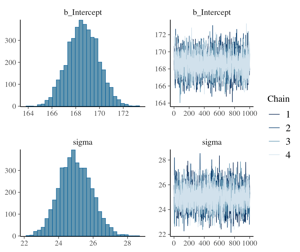
summary(fitresult)
# for above, Rhat should <=1.05,
# Bulk ESS, bulk effective sample size, meausring samping efficiency in the bulk of posterior distribution, that is effective sample size for mean and median
# tail ESS, tail effective sample size, sampling efficiency at the tail of the posterior distribution, that is minimum effective sample size ofr 5% and 95% quantile.
# effective sample size less than poste warm-up iteration indicates samples from the chain are not independent. when the effective size is too small, R will give warning, this indicates sampling problems and chains are not mxed well. Minimum szmple size should be 400
# when effective sample size is more than post wam-up iteration, this happens to normally distributed posterior distribution and parameters are less dependent on each other.
# the folowing draws samples from posterior distribution; therefore this draws for the parameters in posterior space
# this is very different from posterior_predict() function which based on the parameters to make prediction of future data sets
# if during brm model fitting, you set sample_prior="only", then as_draws_df(fitresult_priorOnly) will give you parameter sampling from prior distribution
as_draws_df(fitresult)
as_draws_df(fitresult)$b_Intercept %>% median()
as_draws_df(fitresult)$sigma %>% quantile(c(0.025,0.975))
as_draws_df(fitresult)$sigma %>% sd()
# plot the density of parameters and traceplots showing convergence of chain
plot(fitresult)
Prior Predictive Distribution
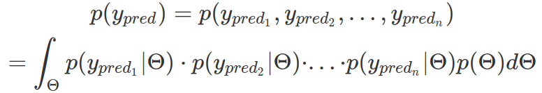
To understand assumptions made about parameters by prior distributions and to check how realistic priors are, it is a good practice to generate prior predictive distributions. Formally, we want to draw many probability distributions of multiple predicted data points. Each distribution is based on a likelihood function whose parameters are instances from a vector of priors (vector of multiple-parameter priors). As we sample a large number of parameter sets from priors (therefore, obtaining many likelihood distributions and many data points from each of them) and calculate the density (multi-dimensional) from all data points, we essentially integrate the probability density over the vector of priors. In practice, we do not need to compute probability density from all data points, rather, we can plot density from each likelihood function.
We can manually set up a function to iterate through randomly sampled parameters from prior distributions, assign them to the likelihood function, and retrieve random data points from the likelihood function. This method does not have a convergence problem but is quite slow. A more efficient method is to use map2_dfr from purrr package.
It is also possible to get prior predictive distribution directly via functions in brms. Instead of fitting the model with real data, a non-NA data set should be used and the parameter, sample_prior, is set to “only” in brm() (to sample prior distribution and make plots, see posterior_predictive and pp_check methods below). However, as brms still uses Stan’s Hamiltonian Monte Carlo sampling method, there might be a convergence problem, especially for very uninformative priors.
We can also try different prior distributions in model fitting (with the real data) to assess how sensitive the model is towards different prior distributions. This is called Prior Sensitivity Analysis. When there is enough data and priors are between weighted and realistic priors, the model is less sensitive to the choices of priors and the model is more likely to converge.
###################################
## prior predictive distribution ##
###################################
## Method1 customized function to generate data from samples of prior distributions
sample_normal_distribution=function(data_points_no, sigma_samples, mean_samples){
#setup empty tibble
data_points=tibble(iteration=numeric(0),
sigma=numeric(0),
mean=numeric(0),
datan=numeric(0),
pred_t=numeric(0))
for(i in seq_along(sigma_samples)){
data_points=bind_rows(data_points,
tibble(iteration=i,
sigma=sigma_samples[i],
mean=mean_samples[i],
datan=seq_len(data_points_no),
pred_t=rnorm(data_points_no,mean=mean,sd=sigma)
))
}
return(data_points)
}
nrow(testdata)
sample_n=1000
tic()
priorPredictiveSamples=sample_normal_distribution(nrow(testdata),sigma_samples = runif(sample_n,0,2000),
mean_samples=runif(sample_n,0,60000))
toc()
## Method2 (preferred): use map2_dfr from purrr package
# map2_dfr iterates simultaneously through two lists and input values from each of them into a function
# this function will return a data frame
sample_normal_distribution_purrr=function(data_points_no, sigma_samples, mean_samples){
map2_dfr(mean_samples,sigma_samples,
function(mean,sigma){
tibble(sigma=sigma,
mean=mean,
datan=seq_len(data_points_no),
pred_t=rnorm(data_points_no,mean=mean,sd=sigma))
#within map2_dfr use iteration as id, and as id is always a string, it needs to be converted to numeric
}, .id="iter") %>%
mutate(iter=as.numeric(iter))
}
tic()
sample_n=1000
priorPredictiveSamples2=sample_normal_distribution_purrr(nrow(testdata),sigma_samples = runif(sample_n,0,2000),
mean_samples=runif(sample_n,0,60000))
toc()
## plot for above
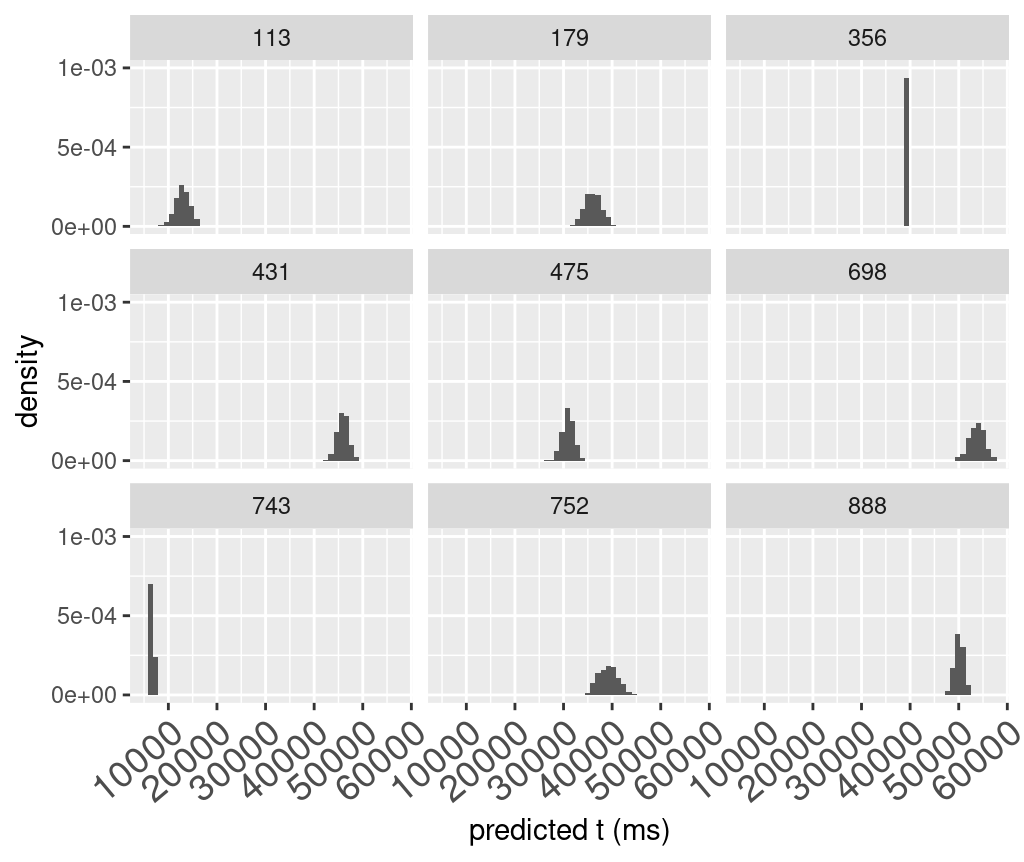
# randomly sample 9 of the sampling numbers ("iter") then plot each of their likelihood density based on the data points sampled
iters=round(runif(9,min=1,max=1000),digits=0)
iters
priorPredictiveSamples2 %>%
filter(iter %in% iters) %>%
ggplot(aes(pred_t))+
# use density other than counts
geom_histogram(aes(y=after_stat(density)),bins=50)+
xlab("predicted t (ms)") +
theme(axis.text.x = element_text(angle = 40,
vjust = 1,
hjust = 1,
size = 14)) +
scale_y_continuous(limits = c(0, 0.001),
breaks = c(0, 0.0005, 0.001),
name = "density") +
facet_wrap(~iter)
# plot summary stats of pred_t
# summary based on "iter", each iter is a set of sigma and mean
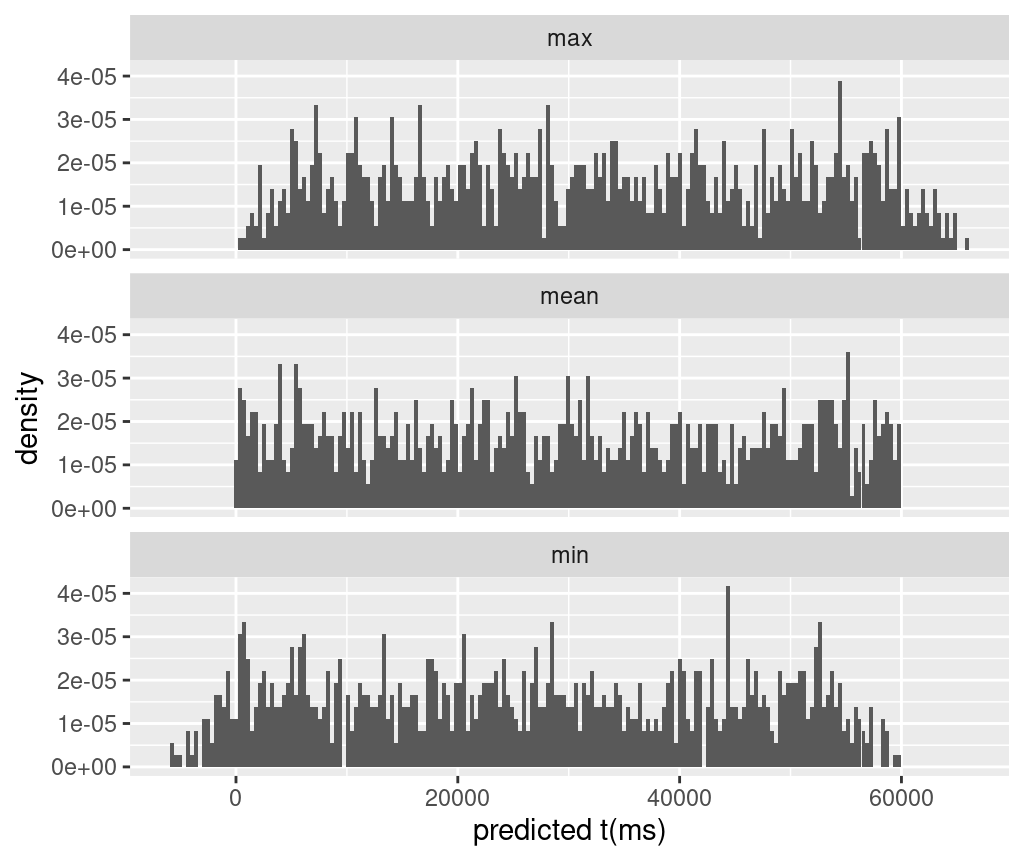
priorPredictiveSamples2 %>%
group_by(iter) %>%
summarise(mean=mean(pred_t),
min=min(pred_t),
max=max(pred_t)) %>%
# select(-iter) %>%
pivot_longer(cols=-iter,names_to="type",values_to="value") %>%
ggplot(aes(value))+
geom_histogram(aes(y=after_stat(density)),bins=200)+
facet_wrap(~type,nrow=3)+
xlab("predicted t (ms)")
## Method3: fit-model with sample_prior="only" while running brm function, then input fitting results into posterior_predict() or pp_check()
# Note: this method might have convergence issue due to iteration/sampling size, priors etc.
# the following prediction is based on prior distribution of parameters
# each set of parameters (sample) as row; data points as columns
posterior_predict(fitresult_priorOnly)
# the following do plots on prior based prediction.
# remember to set prefix="ppd" to ignore and not plotting the real data in the graph.
# for example plots see posterior predictive distribution session
pp_check(fitresult_priorOnly,
type="stat",
stat="mean",
prefix="ppd",
bins=50
)
Posterior Predictive Distribution
Taking the real data, the Bayesian method updates prior distributions of model parameters into posterior distributions. With these, we can sample from the likelihood function for future data points. This is called posterior predictive distribution.
As for prior predictive distribution, we want to sample as many parameter values from posterior distributions as possible, input each set of them into the likelihood function, and randomly retrieve data points from the likelihood. The data points from each likelihood function (with one set of model parameters) or all likelihood functions, give rise to probability distributions or one multi-dimensional distribution of future datasets that we can use to compare with the real data. Therefore, via random sampling, we integrate over the parameters and marginalise them out.

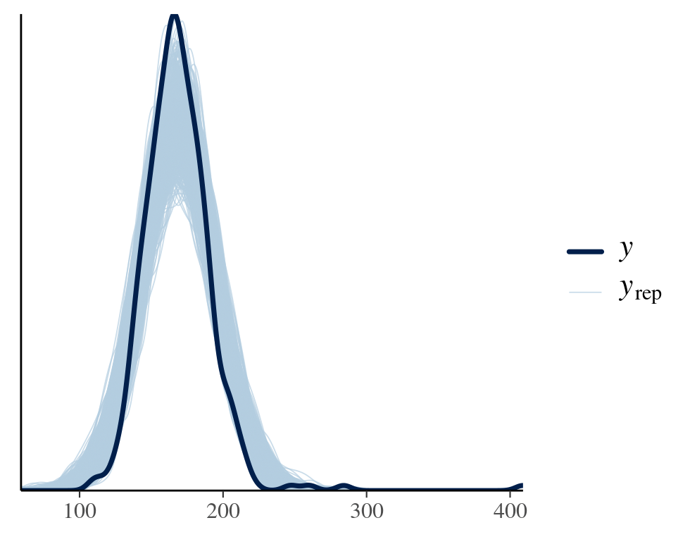
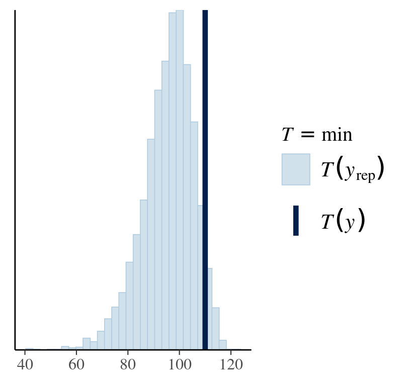
Ideally, posterior predictive distribution should resemble the original data. Although being a perfect fit does not support the model choice, failing to do so is definitely against one. A good model not only produces a good fit but also shows constraints in its predictions.
The function posterior_predict(model_fitting_result) from brms package can directly generate posterior sampling in a data frame with each sample (a parameter-set) as row and data points as columns. When model fitting results are obtained from only prior sampling, this function will return prior sampling. Alternatively, pp_check(model_fitting_result) can directly sample posterior and produce plots of various comparisons. Similarly, pp_check(sample_prior_only_model_result) can also plot prior predictive samples.
#######################################
## posterior predictive distribution ##
#######################################
## method1: use above custom function when sampling from priors:
#   sample_normal_distribution(data_points_no, sigma_samples, mean_samples)
#   remember here the mean_samples and sigma_samples are from posteriors results fitresults
#   if the likelihood function is different from normal, then you should modify this function to sample from corresponding distribution
# Draw parameter samples from posterior distribution by as_draws_df
#   remember, if likelihood is log-normal, then these parameters are on log-transformed unit
posterior_mean_samples=as_draws_df(fitresult)$b_Intercept
posterior_sigma_samples=as_draws_df(fitresult)$sigma

# the following requires 47s
tic()
posteriorPredictiveSamples=sample_normal_distribution(data_points_no=nrow(testdata),
                           sigma_samples=posterior_sigma_samples,
                           mean_samples=posterior_mean_samples)
toc()

## method2: use map2_dfr function built in sample_normal_distribution_purrr and sample from posterior distributions
#   if the likelihood function is different from normal, then you should modify this function to sample from corresponding distribution
# the following requires 4.5s
tic()
posteriorPredictiveSamples_2=sample_normal_distribution_purrr(data_points_no=nrow(testdata),
                                                      sigma_samples=posterior_sigma_samples,
                                                      mean_samples=posterior_mean_samples)

toc()

## method3: use posterior_predict() from brms to get predicted observations
#   rows are parameter sample sets; coloumns are data points from one likelihood
?posterior_predict()
posteriorPredictiveSamples_3=posterior_predict(fitresult)
posteriorPredictiveSamples_3

# by default pp_check will take 10 samples (parameter sets), and default plot is "dens_overlay"
#   this is a wrapper on bayesplot
pp_check(fitresult,ndraws=1000,type="dens_overlay")
pp_check(fitresult,ndraws=12,type="hist")
pp_check(fitresult,type="stat",stat="min")