Extreme Gradient Boosting (XGBoost)

XGBoost is based on an ensemble of gradient boosted trees. It is a supervised learning method where the algorithm tries to optimise model parameters with training data set (features and label), by minimizing the output of the objective function that consists of a Loss function (L) and a regularization term ().

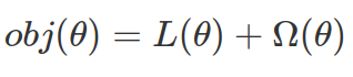
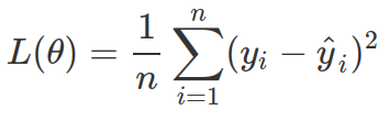
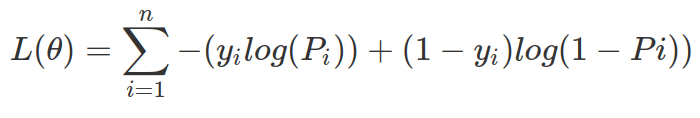
Common choices for L are: mean square error (MSE) or logistic loss for logistic regression.

The regularization term () aims to avoid over-fitting by penalizing complex models. We all want simple and predictive models, however there is always a bias-variance trade-off between these two desires.

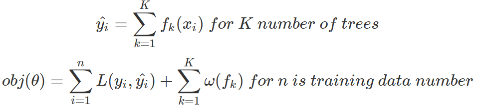
Tree ensemble model consists of a set of classification and regression trees (CART), in which a real score is associated with each leaf. This is very different from decision trees where leaves contain only decision values. For tree ensemble model, we sum the predictions from multiple trees together as final prediction value (where as in decision tree model, it takes the majority votes.). And the objective is to minimize loss function and reducing tree complexity.

In tree boosting ensemble model , tree training is not only additive but also sequential. Each new tree is added at a time and each additional tree optimizes the objective.

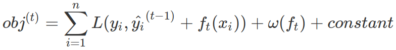
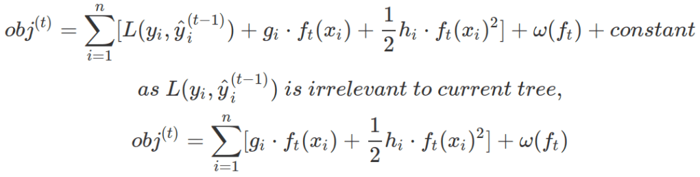
Therefore, at a specific time point, when we only want to optimize the new tree at time t, objective function is:

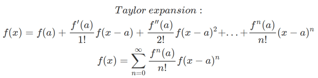
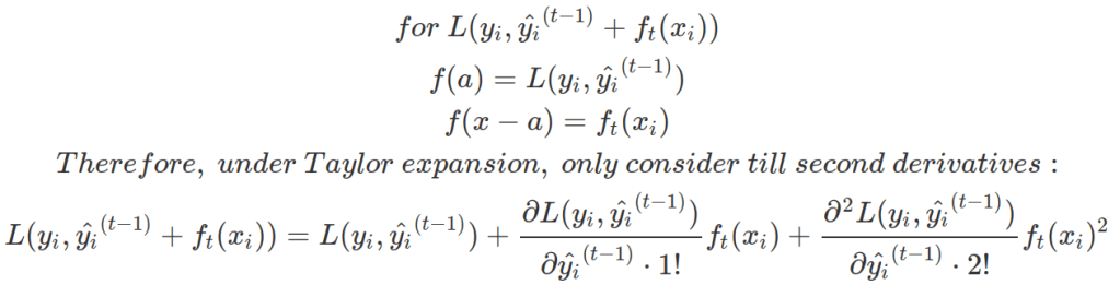
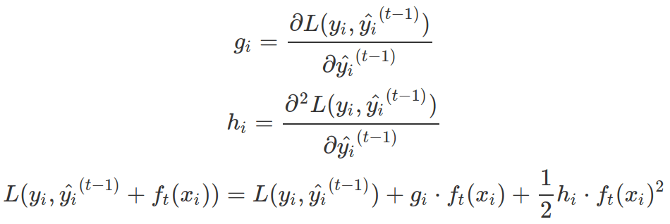
With Taylor expansion, the above objective function for new tree only dependent on term g and h for each data point in training set.

A tree is defined as a vector of scores stored on its leaves. For the following equation q is the function to assign each data point to a corresponding leaf. T is the number of leaves of that tree. Note, in this formula, it is “w” not omega.

The regularization term for each tree depends on the number of leaves and sum of squared leaf scores. Not in this formula, we use omega for regularization term and “w” for vector of leaf scores.

If we represent each tree as its leaf-score vector , the objective function for new tree at time t will be further modified. Data points at the same leaf will have the same leaf-score (w), but they might have different g and h score, due to possibility of being on different leaves in the previous tree. For following formula, n is the number of data points in training set, T is the number of leaves, andis the vector of indexes of all data points belonging to jth leaf.

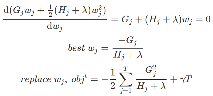
As each leaf is independent from other leaves, the optimisation is on each leaf level, dependent on Gj and Hj of the data points belongs to each leaf. We can find the best leaf-score based on above objective function via first order derivatives on wj. And from wj, we can measure how good the tree is via the obj formula.

XGBoost optimises trees one level at a time. At each tree level, at each leaf, it decides whether splitting it making sense, by calculating whether the gain from the new left leaf and new right leaf taking away the original leaf’s objective score is more than the penality on the new leaf (). If it is smaller than penality (meaning new objective score will be bigger), then new branch will not be added.

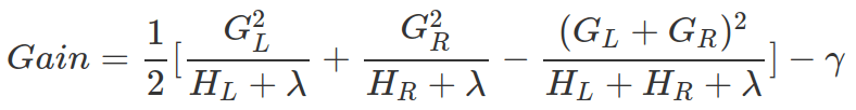
In practice, at each leaf level, XGBoost ranks the data points belongs to this leaf, and calculates all possible Gains (or reductions on objective function) of all different splits.