Logistic Regression

Logistic regression is a generalized linear model (GLM) that defines a link function to connect the output from linear regression to the quantity of interest. Specifically, logistic regression uses the log odds to translate the unbounded real number from the linear regression to a probability between zero and one.

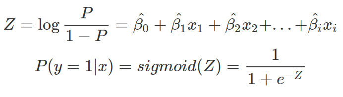
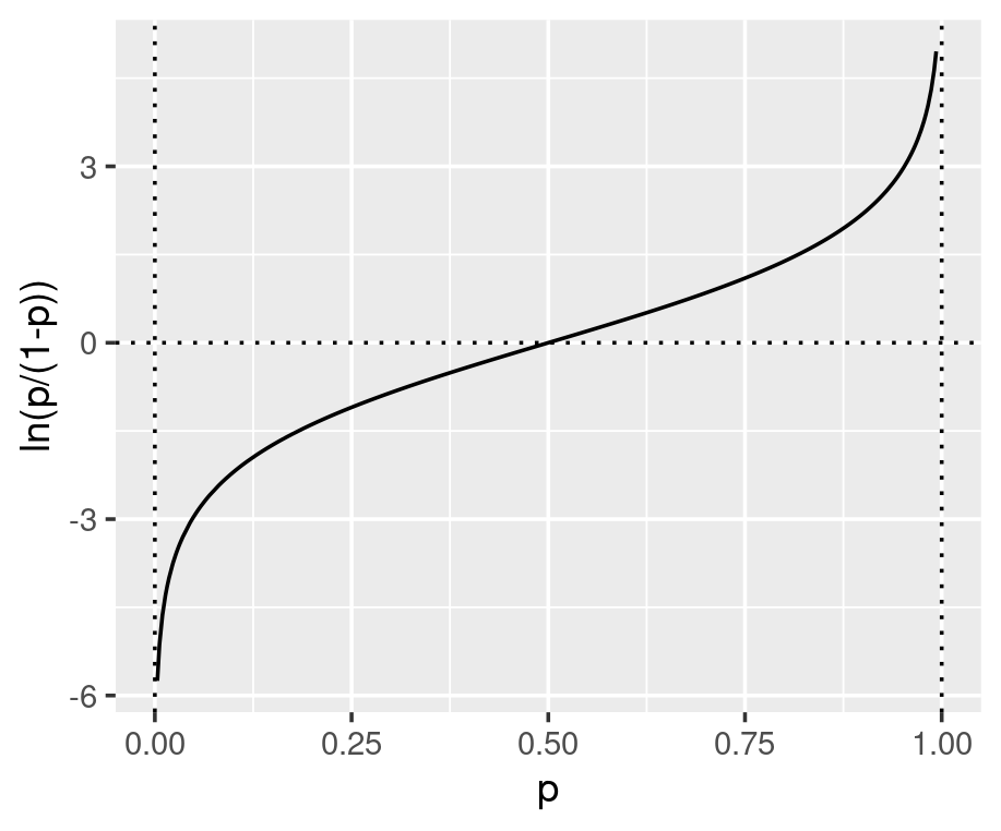
The parameters inside the linear equation are not directly related to the probability, but the log-odds. The relationship between the probability and the output from linear regression is not linear or logarithmic, but logistic. Function qlogis(prob) and plogis(log-odds) can convert probability and log-odds. The conversion from log-odds to probability, after model fitting, is crucial for the interpretation of betas. In a logistic regression model, effectors (x) do not linearly affect the probability. Every unit increase of each effector does not result in the same rise or decrease in probability (see this blog for more details).

In Machine Learning, Logistic regression is a supervised learning method for classifying input data, based on their features, into discrete classes (despite having “regression” in its name). It is mostly used for binary classification. It learns from the training data with given features (input multivariate variables) and labels (output classes), hence the “supervise” part in the name.

Logistic regression classifies input data by estimating its probability of being in one class (only) and users will set the threshold probability (or probabilities) for deciding which one of the two or many classes this input belongs to. The probability, as indicated above, is the logistic conversion of a linear regression of input features.

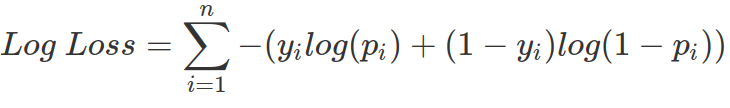
The objective for logistic regression to achieve, while estimating all thes, is to reduce the output from Log-Loss function with its computed probabilities (p) and the true label in the training data set (y). Therefore, logistic regression tries to achieve high probabilities (high log(p), and low -log(p)) for data belong to y=1 class; low probabilities (so high log(1-p), and low -log(1-p)) for data belong to y=0 class.

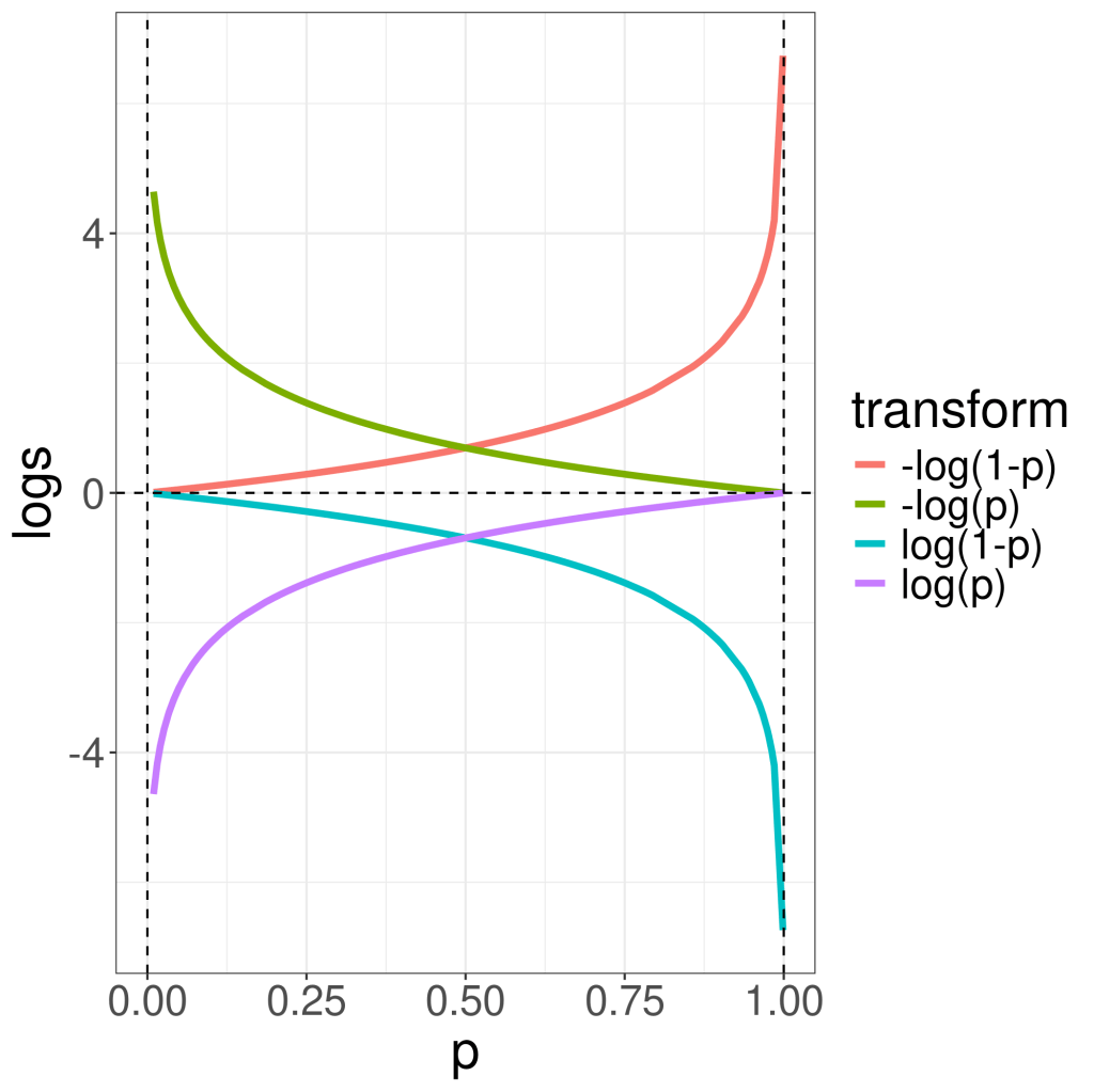
Given p is between, not include, 0 and 1, the following transformation indicates what logistic regression tries to achieve for data belongs to each class. When data truly belongs to y=1 class, logistic regression tries to minimize -log(p) (the green curve); when data’s true label is 0, logistic regression tries to minimize -log(1-p) (the red curve). Note the output from log-loss function ranges from 0 (inclusive) to infinity. The ideal output from logistic regression is to have p approaches 0 for y=0 class, and p is close to 1 for y=1 class, in order to have close-to-zero loss function output.

The above Log Loss function can also be written in terms of Z.

s can be estimated by gradient-decent or maximum-likelihood-estimation (MLE). For gradient decent, parameters are updated iteratively moving towards the direction that decreases the loss (or opposite of the gradient or partial-derivatives on each ) by scales defined by learning rate (or step size). For MLE, the goal is to find all s that maximize Log-Likelihood (equivalent to the negative of the above Log-Loss function). We can achieve this by setting the partial derivative for eachequals to 0 and finding the value of by solving this equation.

The interpretation of in logistic regression is not straightforward. s are considered as log-odds. Odds is calculated as the probability of a desirable outcome over the probability of none-desirable outcomes (P/1-P). And log-odds is logged odds. Therefore to transform log-odds back to odds, you can use exponential function or other power functions dependent on the base of the log. Therefore, indicates the change for odds ratio per unit change of x (the feature having the coefficient of ). And is the odds when all features are 0. Therefore, the baseline probability for desirable outcome is /(1+).