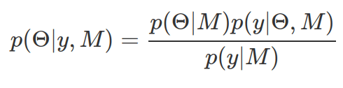
In Bayesian data analysis, we often hypothesize the observed data is sampled from an underlying data model (M) with its own probability density function (PDF) and associated parameters (![]() , such as p in Binomial distribution). The PDF is used as the likelihood function (p(y|
, such as p in Binomial distribution). The PDF is used as the likelihood function (p(y|![]() , M). Our assumption or knowledge or belief about parameters used in the PDF forms the prior distribution (probability distribution of parameter sets to capture the uncertainty. p(
, M). Our assumption or knowledge or belief about parameters used in the PDF forms the prior distribution (probability distribution of parameter sets to capture the uncertainty. p(![]() |M)). These together give rise to the posterior-distribution about these parameters conditioned on the observed data and underlying data model (p(
|M)). These together give rise to the posterior-distribution about these parameters conditioned on the observed data and underlying data model (p(![]() |y, M)). It can also be considered as updated knowledge or belief about these parameters in the PDF, given the data collected. To derive a valid posterior probability distribution, the area under curve needs to be 1. Therefore, the marginal likelihood (p(y|M)) is used to normalize posterior probability.
|y, M)). It can also be considered as updated knowledge or belief about these parameters in the PDF, given the data collected. To derive a valid posterior probability distribution, the area under curve needs to be 1. Therefore, the marginal likelihood (p(y|M)) is used to normalize posterior probability.
When a PDF or PMF is used as a likelihood function, the data is not variable any more. Instead, the data is fixed whereas the parameters in the PDF/PMF are variables. For instance, if we assume the data is drawn from a Binomial distribution. The number of success in the PMF of Binomial distribution is fixed from the data, and the probability of a successful event becomes a variable. Bayesian statistics treats ![]() as a set of variables with associated PDFs/PMFs, other than fixed values, by assigning prior distributions to
as a set of variables with associated PDFs/PMFs, other than fixed values, by assigning prior distributions to ![]() . This is the major difference between Bayesian statistics and the frequentist methods. Bayesian associates uncertainties to these parameter-turned variables, other than deriving fixed values for them via maximum likelihood estimate (MLE). The goal of Bayesian statistics is to find out how we can use Bayes rule to find posterior distributions of
. This is the major difference between Bayesian statistics and the frequentist methods. Bayesian associates uncertainties to these parameter-turned variables, other than deriving fixed values for them via maximum likelihood estimate (MLE). The goal of Bayesian statistics is to find out how we can use Bayes rule to find posterior distributions of ![]() and how we can use data to modify our prior belief about
and how we can use data to modify our prior belief about![]() .
.
Marginal likelihood is derived by integrating out parameters in the likelihood function. Mathematically, this means to have a weighted sum of the likelihood, weighted by the prior plausible values of the parameters involved in likelihood function.
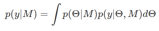
Marginal likelihood is a single number representing the likelihood of observing data (y) given the statistical model (M) after integrating out model parameters. A good model that makes good prediction on data should generate higher marginal likelihood. A poorer/lower marginal likelihood usually is due to too wide prior distribution or too many model parameters. Note, for likelihood function of continuous variables, the derived marginal likelihood does not indicate probability (but likelihood), only in discrete case it gives us probability. Therefore the impact of marginal likelihood is on its relative value to another marginal likelihood of the same data however by different Model — that is called Bayes Factor.
In the following examples, we assume that we observe 70 heads in 100 coin tosses. However we are not sure whether this coin is a fair coin, that is to say we do not know the probability of getting a head in each coin flip. We will use different statistical distributions to model coin tosses, as likelihood functions, with different numbers of parameters involved (one parameter, p, for binomial distribution; two of the three parameters, ![]() and
and ![]() , for beta-binomial distribution). We will also vary the prior distributions, in order to explore their impacts on the marginal likelihood. As you can see that a “flat”/uninformative prior or a likelihood function containing many parameters may have less support from the data.
, for beta-binomial distribution). We will also vary the prior distributions, in order to explore their impacts on the marginal likelihood. As you can see that a “flat”/uninformative prior or a likelihood function containing many parameters may have less support from the data.
# install.packages("extraDistr")
library(extraDistr)  #to use dbbinom()

## Marginal likelihood for different priors and likelihood functions ##
#     In order to show that likelihood with broader prior, or likelihood function with many parameters, has small marginal likelihood and does not make good predictions on data.

## Model1: beta(5,3) as prior with binomial as likelihood
# set up the function representing likelihood function with a specific parameter value, multiplied by the probability of that parameter reflected in prior distribution
lp1=function(p){
  dbinom(x=70,size=100,prob=p)*dbeta(x=p,shape1=5,shape2=3)
}
# integrate the above function over all possible p between 0 and 1.
mlikeli1=integrate(f=lp1,lower=0,upper=1)$value
mlikeli1 #0.021

## Model2: un-informative beta(1,1) with binomial
lp2=function(p){
  dbinom(x=70,size=100,prob=p)*dbeta(x=p,shape1=1,shape2=1)
}
mlikeli2=integrate(f=lp2,lower=0,upper=1)$value
mlikeli2  #0.01, less good as mlikeli1, as here the prior is very flat

BF12=mlikeli1/mlikeli2 #2.2

## Model3: log-normal for prior with beta-binomial for likelihood
# beta-binomial (f(x|n,a,b)) usually has 3 paraemters, here as we know n is 100, we will model only a and b with log-normal distributions for priors
lp3=function(a,b){
  dbbinom(x=70,size=100,alpha=a,beta=b)*
    dlnorm(x=a,meanlog=0,sdlog=100)*
    dlnorm(x=b,meanlog=0,sdlog=100)
}
# first integrate alpha, for every given b
mlikeli_ona=function(b){
  #change lp3 into a function of a
  integrate(function(a) lp3(a,b), lower=0, upper=Inf)$value
}

# integrate beta
mlikeli3=integrate(Vectorize(mlikeli_ona),lower=0,upper=Inf)$value
mlikeli3  #4.3e-6, worst performing of all three as there are more parameters in likelihood function, so can not has least support from the data.

BF13=mlikeli1/mlikeli3 #5075
BF23=mlikeli2/mlikeli3 #2286

#### extra ####
# explore prior distribution
ggplot()+
  geom_line(data=tibble(p=seq(0,1,by=0.001),d=dbeta(p,5,2)),aes(x=p,y=d),color="black")+
  geom_line(data=tibble(p=seq(0,1,by=0.001),d=dbeta(p,1,1)),aes(x=p,y=d),color="red")+
  theme(text=element_text(size=30))

ggplot()+
  geom_line(data=tibble(p=seq(0,1,length.out=1000),d=dlnorm(p,meanlog=0,sdlog=100)),aes(x=p,y=d))+
  theme(text=element_text(size=30))

# explore likelihood*prior function
ggplot()+
  geom_line(data=tibble(p=seq(0,1,by=0.001),d=lp1(p)),aes(x=p,y=d),color="black")+
  geom_line(data=tibble(p=seq(0,1,by=0.001),d=lp2(p)),aes(x=p,y=d),color="red") #+
  # you can not plot lp3 here, even if beta is fixed, as alpha will go beyond 1
  geom_line(data=tibble(a=seq(0,1000,by=1),d=lp3(a,20)),aes(x=a,y=d),color="green")
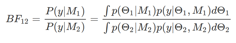
Bayes Factor (BF) is a measure of relative evidence quantified by the ratio of marginal likelihoods. It is a tool, in Bayesian statistics, to test hypothesis, comparing any kind of hypothesis/models, via quantifying evidence provided by data in support of one model or another. A bigger BF indicates M1 more favoured by evidence than M2. For above example, BF12 is 2.2, BF13 is 5075 and BF23 is 2286. There is also a scale proposed by Jeffreys (1939) for Bayes Factor strength, in which 3-10 provides moderate evidence, 10-30 provides strong evidence, and >30 shows very strong evidence for model whose marginal likelihood is on the numerator part of the BF. This model comparison method is very different from the likelihood-ratio of frequentist method. Because here, the ratio is independent from model parameter, as all prior parameter values are taken into account simultaneously.
Bayes Factor is very sensitive to prior assumptions of model parameters, therefore some suggest to use default prior distributions, where prior parameters are fixed. It is not recommended, although widely used.
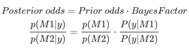
Bayes Factor shows data evidence in favour of one model over another. It tells us the amount by which we should update our relative belief between two models in light of the data and prior knowledge of parameter ranges. However, BF does not tell us which model is more probable. To know how much more probable M1 is than M2 , we need prior odds and BF, in order to calculate the posterior odds.
Typically, for Bayesian analysis, we visualize prior, likelihood and posterior distribution together, provided they are all scaled to integrate to one. We can also summarize posterior distribution by computing mean (value of expectation), the variance, and showing the parameter range giving 95% credible interval.
As mentioned in this post, posterior distribution is a compromise between prior and likelihood. And which of the two influences posterior most, depends on how great the certainty is reflected in the prior and how much data is collected.
Finally, posterior distribution can be used as new prior for further analysis to incrementally gain the knowledge/information.
