Beta-binomial distribution is a discrete probability distribution. It is basically a Binomial distribution when probability of success at each of the “future” n Bernoulli trials is not fixed but drawn from a Beta distribution.
Beta-binomial distribution is used to capture overdispersion in Binomial type distributed data.
There are 3 parameters in Beta-binomial: n, the future total trials; ![]() , the number of known successes;
, the number of known successes; ![]() , the number of known failures. The variable k in Beta-binomial distribution is the number of success in the n trials. The probability mass function (PMF) is as following and beta() is the beta function.
, the number of known failures. The variable k in Beta-binomial distribution is the number of success in the n trials. The probability mass function (PMF) is as following and beta() is the beta function.

In R, we use dbbinom(x, size, alpha, beta) from the “extraDistr” package to model Beta-binomial’s PMF and pbbinom(q, size, alpha, beta) and rbbinom(n, size, alpha, beta) for CDF and random sampling.
# install.packages("extraDistr")
library(extraDistr) #to use dbbinom()
################################
## Beta-binomial distribution ##
################################
# fix n
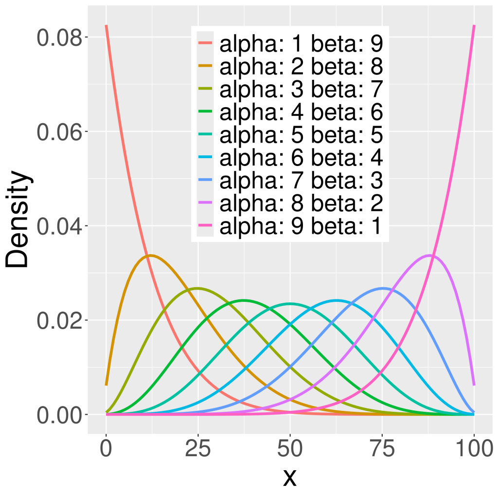
n=100
# define sequence for alpha and beta
a_b_total=10
a=seq(1,9,by=1)
b=a_b_total-a
# defie x, how many successes within n
x=seq(0,100,by=1)
# calculate density for each alpha, beta combination as columns
data2plot=tibble(x=x)
for(i in 1:length(a)){
name=paste0("alpha: ",a[i]," beta: ",b[i])
print(name)
data2plot=data2plot %>%
dplyr::mutate(!!name := dbbinom(x,size=n,alpha=a[i],beta=b[i]))
}
data2plot=pivot_longer(data2plot,cols=-x,values_to = "density",names_to = "type")
# plot
ggplot(data=data2plot)+
geom_line(aes(x=x,y=density,color=type),size=1.3)+
scale_y_continuous(name="Density")+
theme(text=element_text(size=30),
legend.position = c(0.5,0.7),
legend.title=element_blank())
ggsave("./plots/Beta_Binomial_PMF_alter_alpha_beta.png")
