Univariate distributions display probability distribution for one variable, such as the number of desirable events in Binomial distribution, the variable having mean and standard deviation in Normal distribution, and the probability for each Bernoulli event in a Beta distribution. A bivariate or multivariate distribution defines probability for two or more dimensions.
Assuming a PMF is defined by two discrete variables x and y. The density plot is shown below and density values are in the following table. The sum of all densities equals approximately to 1.
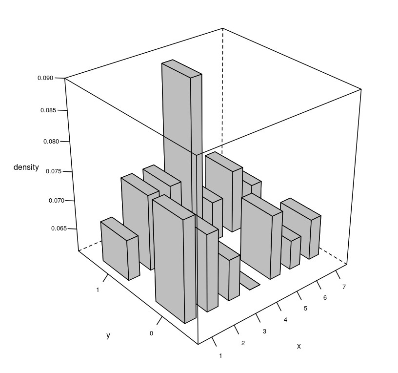
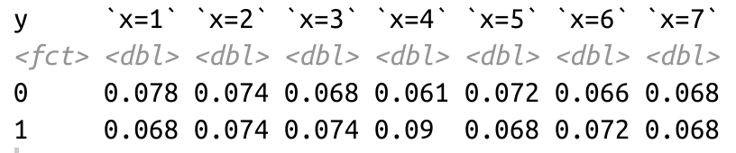
Three important concepts:
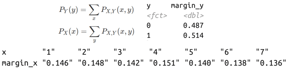
1. Marginal Distribution of y and x:
Essentially, the marginal distribution of y is derived by summing up all densities corresponding to all x values for each individual value of y (sum up each row, and derive the value on the “margin” for each row). Correspondingly, the marginal distribution of x is calculated by summing up all densities of y values for each x (sum up each column, and write the value on the “margin” below each column).
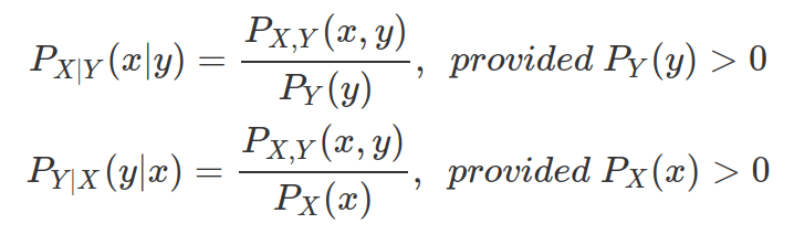
2. Conditional distributions:
Conditional distribution of x dependent on y is calculated by the probability density of each pair of x and y, divided by the density of y (the value correspond to y in the pair) in the marginal distribution of Y, and vice versa. Therefore, the resulting distribution maintain the exact dimensionality of the original PMF. For the following tables, the first one is conditional distribution on y and second one is on x.


3. Covariance and Correlation:
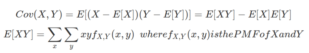
If there is a high probability that large values of a random variable X are associated with large values of another random variable Y, we say that the covariance between X and Y are positive. Cov(x,y)>0.
Cov(X,Y) = E[(X – E[X])(Y – E[Y])], where E[.] is expectation of Value, also known as mean. Cov(X,Y) = E[XY – YE[X] – XE[Y] + E[X]E[Y]] = E[XY] – E[Y]E[X] – E[X]E[Y] + E[X]E[Y] = E[XY]-E[X]E[Y]
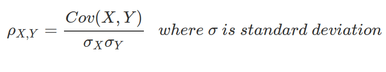
The correlation between the two random variables X and Y are defined as following. This also means that when covariance between two variables is zero, the correlation is zero.
#### Bivariate distribution ####
### Discrete Bivariate distribution ###
library(ggplot2)
library(tibble)
library(tidyr)
## set up alias ##
group_by=dplyr::group_by
summarise=dplyr::summarise
mutate=dplyr::mutate
filter=dplyr::filter
select=dplyr::select
case_when=dplyr::case_when
########################################
#1 generate discrete values for x and y
x=sample(1:7,2000,replace=T)
y=sample(0:1,2000,replace=T)
data=tibble(x=x,y=y)
data
#2 calculate density
density_data=data.frame(table(data)) %>%
dplyr::mutate(density=round(Freq/sum(Freq),digits=3))
density_data
sum(density_data$density)
#3 plot density
# install.packages("latticeExtra")
library("latticeExtra")
cloud(density~x+y, density_data, panel.3d.cloud=panel.3dbars, col.facet='grey',
xbase=0.5, ybase=0.5, scales=list(arrows=FALSE, col=1),
par.settings = list(axis.line = list(col = "transparent")))
# alternative 2d plot
ggplot(density_data, aes(x, y, fill = density)) +
geom_tile() +
scale_fill_fermenter(type = "div", palette = "RdYlBu")
#4 display table
density_data_wide=density_data %>%
pivot_wider(id_cols=y,names_from=x,values_from=density) %>%
setNames(c("y","x=1","x=2","x=3","x=4","x=5","x=6","x=7"))
density_data_wide
#5 calculate marginal distribution for y
density_data_margin_y=density_data %>%
group_by(y) %>%
summarise(margin_y=sum(density))
density_data_margin_y
density_data_margin_x=density_data %>%
group_by(x) %>%
summarise(margin_x=sum(density))
density_data_margin_x %>% t()
#6 calculate conditional distribution
density_data_condition_on_y=density_data %>%
mutate("x|y"=case_when(y==0~density/(density_data_margin_y %>% filter(y==0))$margin_y,
y==1~density/(density_data_margin_y %>% filter(y==1))$margin_y,
TRUE~0)) %>%
pivot_wider(id_cols=y,names_from=x,values_from=`x|y`) %>%
setNames(c("y","x=1","x=2","x=3","x=4","x=5","x=6","x=7"))
density_data_condition_on_y
density_data_wide
density_data_margin_y
density_data_condition_on_x= density_data %>%
mutate("y|x"=case_when(x==1~density/(density_data_margin_x %>% filter(x==1))$margin_x,
x==2~density/(density_data_margin_x %>% filter(x==2))$margin_x,
x==3~density/(density_data_margin_x %>% filter(x==3))$margin_x,
x==4~density/(density_data_margin_x %>% filter(x==4))$margin_x,
x==5~density/(density_data_margin_x %>% filter(x==5))$margin_x,
x==6~density/(density_data_margin_x %>% filter(x==6))$margin_x,
x==7~density/(density_data_margin_x %>% filter(x==7))$margin_x,
TRUE~0)) %>%
pivot_wider(id_cols=y,names_from=x,values_from=`y|x`) %>%
setNames(c("y","x=1","x=2","x=3","x=4","x=5","x=6","x=7"))
density_data_condition_on_x
density_data_wide
density_data_margin_x
#7 calculate covariance and correlation
cov(data$x,data$y)
cor(data$x,data$y)
sd(data$x)
sd(data$y)
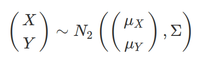
cov(data$x,data$y)/(sd(data$x)*sd(data$y))For two continuous variables X and Y, each of which comes from a normal distribution. Their bivariate distribution is defined in terms of their means, standard deviations and correlation between them. The joint distribution of X and Y is defined as:
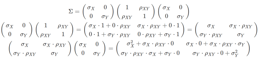
![]() is variance-covariance matrix:
is variance-covariance matrix:
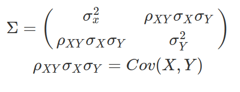
A variance-covariance matrix can be decomposed into a diagonal matrix of standard-deviations multiplies correlation matrix, then multiplies the diagonal matrix of standard-deviations again (see following demonstrations). Remember in matrix multiplication, you can not swap the order of matrices. In matrix multiplication, the first matrix’s column number need to be the same as the row number of the second matrix. The resulting new matrix has a row number of the first matrix and column number of the second (a 2×3 matrix multiplies a 3×4 matrix, the result matrix is 2×4). The first row of the new matrix is the result of first row of matrix1 sum-multiplying each column of matrix2 (sum-multiplying: imagine you transpose the first row of matrix1 into a one column matrix, then each of its element multiplying the corresponding element in a column of matrix2, then sum the result together). In R, matrix multiplication is achieved by %*%.
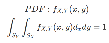
The PDF of above distribution has area under curve equals to 1. CDF calculates the probability of having X less than u and Y less than v.

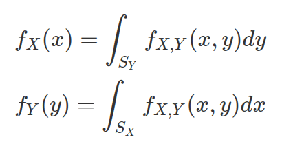
The marginal distribution can be derived by marginalizing out (via integration) the other random variable as following. The conditional probability (e.g. X|Y) will be calculated by diving density by marginal distribution of the conditioned probability ( in this case,  )
)
Generating continuous bivariate data in R requires knowing the mean values and variance-covariance matrix (therefore their standard-deviations and correlation). You can randomly sample from bivariate/multivariate distribution by using mvrnom(n, mu, Sigma) function from MASS library.

library(ggplot2)
library(tibble)
library(tidyr)

######### Continuous Bivariate distribution ##############
#install.packages("MASS")
# if (!require("BiocManager", quietly = TRUE))
#   install.packages("BiocManager")
# BiocManager::install("nloptr")
# install.packages("ggpubr")
library(MASS)
library(ggpubr)

# Assuming we want to define and smpling 100 pair of data points from a bivariate distribution, having the following properties:
rho=0.8
mu_x=0
mu_y=0
sigma_x=6
sigma_y=12

#1 define variance-covariance matrix
big_sigma=matrix(data=c(sigma_x^2,rho*sigma_x*sigma_y,rho*sigma_x*sigma_y,sigma_y^2),nrow=2,byrow=TRUE)
big_sigma

#2 sampling data by mvrnorm()
dataPair=mvrnorm(n=100,mu=c(mu_x,mu_y),Sigma=big_sigma)
dataPair #in matrix format

# plot dataPair and check correlation
cor(dataPair)
dataPair=tibble(dataPair)
colnames(dataPair)=c("x","y")
dataPair

p=ggscatter(dataPair,x="x",y="y",
          add="reg.line",
          conf.int=TRUE,
          color="red",
          fill="gray",
          rug=TRUE,
          )+
  stat_cor(label.x=-10,size=9)+
  theme(text=element_text(size=24))

ggexport(p,filename="plots/continious_BivariateDistribution.png")

#4 demonstrate the variance-covariance matrix can be the decomposed to three matrices multiplying together: diagonal matrix of standard deviation, correlation matrix, and diagonal matrix of standard deviation
diagonal_sigma=diag(c(sigma_x,sigma_y))
diagonal_sigma
correlation_matrix=matrix(c(1,rho,rho,1),nrow=2,byrow = TRUE)
correlation_matrix

big_sigma==diagonal_sigma %*% correlation_matrix %*% 