A data set can be characterised by its mean value and spread. Mean is also called the expectation of the data and can be computed by the sum of the “weighted” unique values:
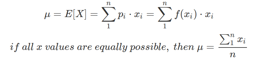
The f(x) is the PMF or PDF of x, showing the possibility of getting each x value. If f(x) is a uniform distribution of x, indicating all x values are equally possible, then the second line of equation is valid.
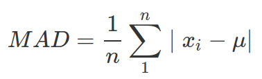
The wider spread of a data set, the more uncertainty there is about the estimate of the mean. The spread of data can be measured by:
- Mean Absolute Deviation (MAD) :
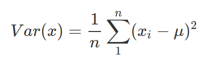
- Variance: similar to MAD, but do not need to work out the absolute value and carries exponential penalty to values deviating greatly from the mean. It is also called sigma squared. Note: when you do not know the population mean(
 ), but only the mean from samples (
 ), then divide by n-1 other than n. The R function, var() calculate variance as sample variance (therefore divided by n-1)
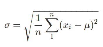
- Standard Deviation: more interpretable than variance. It is also called “sigma”. Note, the same as above, when you do not know the population mean () but mean of the sample (), then divide by (n-1) before taking square root.
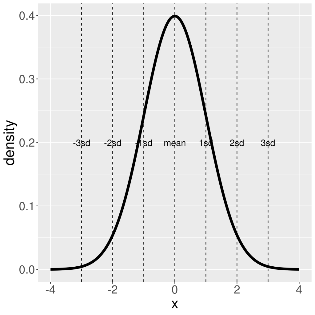
Normal distribution is a continuous probability distribution, taken mean () and ( ) as its only two parameters. Normal distribution shows how strong we believe in our mean. And it shows density of all possible values from
  to
to  . Therefore, when integrate (by using integrate() function in R), you need to provide explicit values for the lower and higher bound (this can be taken as
  ). There are 68% chance ( area under PDF of normal distribution) x value sits between
  , and 95% chance x is between
  , and 99.7% between
  .
.
The probability density function (PDF) of Normal distribution:
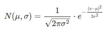
The PDF function for a continuous distribution does not give probability value to a point value of x, whereas the PMF function for discrete distribution does. This is because for continuous distribution, probability corresponds to area under curve and area under a point is 0. Therefore probability need to be computed between two x values and via the CDF function (using CDF twice with the two values separately then calculate difference, alternatively using the integrate function).
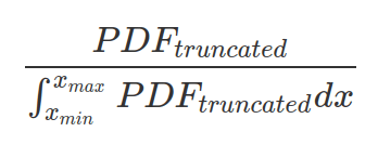
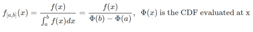
One can truncate a PDF to support a more narrow range of x values (between xmin and xmax). In this case, probability outside this range will be zero. And one should make sure the area under truncated PDF sums up to 1, by dividing the truncated PDF with the area under this PDF.
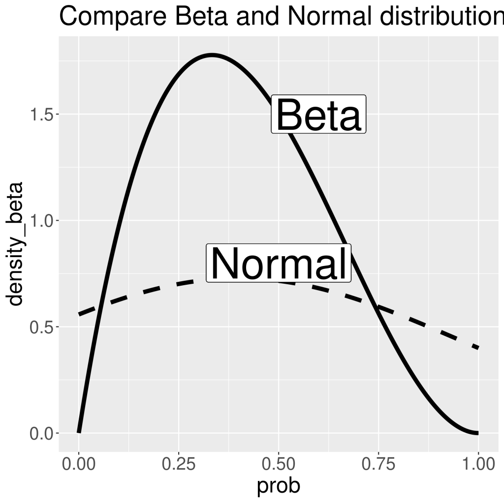
Only use this distribution when the only things you know about the data are mean and standard deviation. Do not try to convert, for instance, Beta distribution, to normal distribution (e.g. Beta(2,5) to normal distribution with mean 0.4 and sigma 0.56, assuming success is 1 and failure is 0 , and sigma is calculated as sample standard deviation). As can be seen in the following plot, the peak of Beta and Normal distributions are similar. However, Normal distribution is much flatter than Beta. It is because its x values has no boundaries. And to have area-under-curve equals to 1, Normal distribution needs to spread out. This also shows that Normal distribution includes impossible values. And in our case, we know x axis should only contain values between 0 and 1, as Beta distribution shows the density of probability of success or failure in each Bernoulli trial. And this probability can only be between 0 and 1.
Useful R functions for Normal distribution:
- Probability Density Function (PDF): dnorm(x, mean=0, sd=1): the probability for a point on x axis. The default value for mean is 0 and sigma is 1.
- Cumulative Distribution Function (CDF): pnorm(x, mean=0, sd=1, lower.tail=TRUE): the area under PDF curve for X<=x, if lower.tail==TRUE, or for X>x when lower.tail==FALSE. You could also get area under PDF between two x values by using integrate(function(x) dnorm(x, mean, sd), [value1], [value2])
- Quantile Function: qnorm(p, mean=0, sd=1, lower.tail=TRUE): reverse function of CDF above. This function returns the x threshold that gives rise to area under PDF curve of p. If lower.tial==TRUE, p corresponds to X<=x, if lower.tail==FALSE, p corresponds to X>x.
- Random sampling of x based on probability density: rnorm(n, mean=0, sd=1): n is the number you want.
- Finding quantile from a vector of data (that you assume follows a normal distribution) or from simulated normal distribution data, e.g. from rnorm: quantile(dataVector, probs=c(0.025,0.975)). This function will return values correspond to probability of 0.025 and 0.975 from the distribution it estimates (so the value returned not necessarily from the dataVector you inputted).
##### Compare Beta and normal distribution ####
library(tidyr)
library(ggplot2)
library(tibble)

## data ##
# change Beta(2,3) to c(1,1,0,0,0)
data=c(1,1,0,0,0)
mean(data)
sd(data)

## understand R function var() and sd() ##
# calculate variance as if this is population or sample
pop_var=sum((data-mean(data))^2)/5
pop_var

sample_var=sum((data-mean(data))^2)/(5-1)
sample_var

#compare with R function var()
var(data)  #calculate sample variance

# calculate sample sd
sample_sd=sample_var^0.5
sample_sd

# compare with R function sd
sd(data)  #sample sd as above

## plot beta and normal distribution ##
p=seq(0,1,0.001)

ggplot(data=tibble(prob=p,density_beta=dbeta(p,2,3),density_norm=dnorm(p,0.4,0.548)))+
  geom_line(aes(x=prob,y=density_beta),linewidth=2)+
  geom_line(aes(x=prob,y=density_norm),linewidth=2,linetype=2)+
  geom_label(x=0.5,y=0.8,label="Normal",size=15)+
  geom_label(x=0.6,y=1.5,label="Beta",size=15)+
  theme(text=element_text(size=22))+
  ggtitle("Compare Beta and Normal distribution")

ggsave("plots/Beta_vs_normal_distribution.png")

## plot normal distribution with mean=0, sd=1
x=seq(-4,4,0.001)
density=dnorm(x,mean=0,sd=1)
max(density)
ggplot(data=tibble(x=x,density=density),aes(x=x,y=density))+
  geom_line(linewidth=2)+
  geom_vline(xintercept = 0 + seq(-3,3)*1, col = "black",lty = 2)+
  geom_text(data=tibble(x=0 + seq(-3,3)*1,y=max(density)/2,label=c(paste0(-(3:1),"sd"),"mean",paste0(1:3,"sd"))), aes(x=x,y=y,label=label),size=5)+
  theme(text=element_text(size=23))

ggsave("plots/normalDistribution_sd.png")

# Area under curve
#between 3 sigma, 99.73%
1-2*pnorm(-3,mean=0,sd=1,lower.tail=TRUE)
#between 2 sigma, 95.4%
1-2*pnorm(-2,0,1,lower.tail=TRUE)
#between 1 sigma, 68.3%
1-2*pnorm(-1,0,1,lower.tail=TRUE)

# plot CDF for above normal distribution
x=seq(-4,4,0.001)
cumulativeDensity=pnorm(x,mean=0,sd=1, lower.tail=TRUE)

ggplot(data=tibble(x=x,CD=cumulativeDensity),aes(x=x,y=cumulativeDensity))+
  geom_line(linewidth=2)+
  geom_vline(xintercept = 0 + seq(-3,3)*1, col = "black",lty = 2)+
  geom_text(data=tibble(x=0 + seq(-3,3)*1,y=max(cumulativeDensity)/2,label=c(paste0(-(3:1),"sd"),"mean",paste0(1:3,"sd"))), aes(x=x,y=y,label=label),size=5)+
  theme(text=element_text(size=23))

ggsave("plots/normalDistribution_cdf.png")
Truncated Normal Distribution
Any distribution can be truncated within a boundary. However, as a valid probability distribution, the area below the probability density curve, or the sum of probability mass, should be integrated into one. Therefore the new PDF or PMF should be normalised by the area or sum within these boundaries.
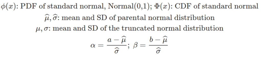
A truncated normal distribution can be defined by dtnorm (PDF), ptnorm (CDF), qtnorm (quantile) and rtnorm function from the extraDistr package. The mean and standard deviation used within these functions are mean and SD of the parental, none-truncated distribution, not of the truncated one.
Unless the truncated normal distribution is symmetric, the new mean does not coincide with the parental one. The standard deviation of any truncated distribution does not coincide with the parental one. The following equations can help to calculate the mean and standard deviation for the truncated normal distribution based on their values in the parental distribution.
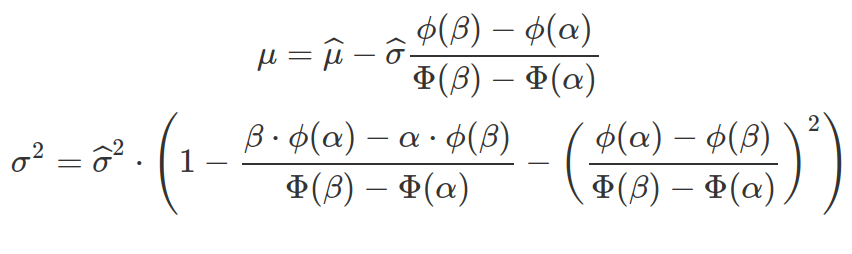
Sometimes, observations are derived from the truncated distribution and we need to work out the mean and standard deviation of the parental, none-truncated distribution to define the truncated one. The above two equations can be written based on the specifications for multiroot() function in the rootSolve package.
#####################################
### Truncated Normal Distribution ###
#####################################
packs=c("brms","rstan","bayesplot","dplyr","purrr","tidyr","ggplot2","ggpubr","extraDistr","sn","hypr","lme4","rootSolve","bcogsci","tictoc")
lapply(packs, require, character.only = TRUE)

## calculating truncated mu and sd from parental ones
# boundaries
a = 0
b = 600
# parental mean and sd
bar_mu = 300
bar_sigma = 200
# intermediate variables
alpha = (a - bar_mu) / bar_sigma
beta = (b - bar_mu) / bar_sigma
# intermediate terms
term1 = ((dnorm(beta) - dnorm(alpha)) /
            (pnorm(beta) - pnorm(alpha)))
term2 = ((beta * dnorm(beta) - alpha * dnorm(alpha)) /
            (pnorm(beta) - pnorm(alpha)))
# the mean and sd of the truncated distribution
mu = bar_mu - bar_sigma * term1
sigma = sqrt(bar_sigma^2 * (1 - term2 - term1^2))

## calculate parental bar_mu and bar_sigma from truncated observations
# set up equation system for multiroot
#   parms are known boundaries a, b and truncated mu and sigma
#   x are data, from which can calulate x[1] parental mu, and x[2] prental sigma
eq_system = function(x, parms) {
  mu_hat = x[1]
  sigma_hat = x[2]
  alpha = (parms["a"] - mu_hat) / sigma_hat
  beta = (parms["b"] - mu_hat) / sigma_hat
  # both F1 and F2 are equations equals to zero
  c(F1 = parms["mu"] - mu_hat + sigma_hat *
      (dnorm(beta) - dnorm(alpha)) /
      (pnorm(beta) - pnorm(alpha)),
    F2 = parms["sigma"] -
      sigma_hat *
      sqrt((1 - ((beta) * dnorm(beta) -
                   (alpha) * dnorm(alpha)) /
              (pnorm(beta) - pnorm(alpha)) -
              ((dnorm(beta) - dnorm(alpha)) /
                 (pnorm(beta) - pnorm(alpha)))^2)))
}

# in reality, x is from observation that we believe are truncated from a normal distribution
# for this exercise, use randomly sample values
x = rtnorm(10000000, mean = 300, sd = 200, a = 0, b = 500)

# solve algebra for parental parameters
soln = multiroot(f = eq_system,
                  start = c(1, 1),
                  parms = c(a = 0,
                            b = 500,
                            mu = mean(x),
                            sigma = sd(x)))
soln$root
