Beta Distribution

Binomial distribution requires the knowledge of the probability for obtaining the desirable outcome in each trial (p). However, in real life, this parameter needs to be inferred from data. The foundation of statistics is inference, that is to figure out the probability from observations.

Beta distribution shows probabilities of a continuous range of probabilities (variable p) of obtaining a fixed number of successes (parameter) and failures (parameter). It helps to infer how likely or unlikely are a range of probabilities for obtaining this amount of successes and failures as we observed. Beta distribution is closely related to binomial distribution. Beta distribution shows how well each binomial distribution (p, k=, n=+) can describe the data observed.

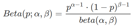
The Probability Density Function (PDF) for Beta distribution is as following. The world “density” indicates this PDF can compute probability for any given probability (of obtaining  and ). And “density”, other than “mass”, indicates this is a continuous distribution.

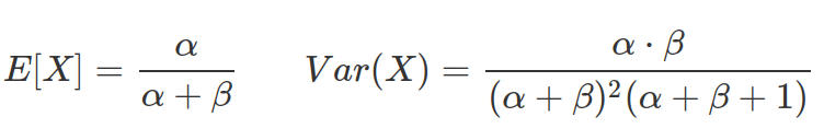
The expectation (mean) and variance of Beta distribution are:

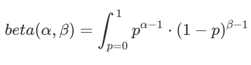
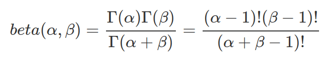
The beta function in the denominator of the PDF of Beta distribution is designed for normalize the density to have area-under-curve equal to 1 (or the sum of all probabilities equals to 1). It is the integration between 0 and 1.

Beta distribution is one of the favourite distributions to use in Bayesian statistics. It is because two Beta distributions are very easy to combine. In the case where both prior distribution and likelihood function are depicted by Beta distributions, the resulted posterior distribution is also a Beta distribution with its being the sum of prior and likelihood’s s and being the sum of the two s. As Beta distribution is normalized in nature, there is no need to normalize the resulted posterior distribution.

The above example is a beta-beta conjugate. And the prior is a conjugate prior. Formally, given likelihood p(y|), if prior p() results in a posterior p(|y) that has the same form as prior distribution (meaning both belongs to the same family of probability distribution), then we call p() a conjugate prior.

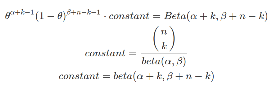
Beta distribution is also a conjugate prior forming Binomial-Beta conjugate. Binomial and Beta distribution have similar kernels, that is the none-constant part the corresponding PMF and PDF (e.g. 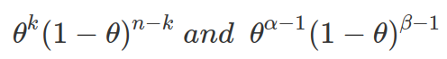). When Binomial distribution is used as the likelihood function and Beta as prior, the resulted posterior distribution is a Beta distribution. And the constant part normalize the posterior distribution, therefore it forms a new beta function.

Useful functions for Beta distribution:

• PDF: dbeta(p, alpha, beta) what is the probability to have a binomial distribution with k=alpha, p, n=alpha+beta. dbeta(p, 1, 1) represent PDF of an uniform distribution.
• CDF: pbeta(p, alpha, beta, lower.tail=TRUE) what is the integrated area under PDF curve from 0 to p inclusive. You can also get this by integrate(function(x) dbeta(x, alpha, beta), 0, p)
• Quantile function: qbeta(cumP, alpha, beta, lower.tail=TRUE) Reverse function of CDF. cumP is the cumulative area (result from CDF) under curve of PDF and the result returned by quantile function would be the threshold p giving rise to this area. As lower.tail=TRUE, the area under PDF curve covers from 0 to p inclusive. You can use quantile function to find median of a distribution. The median probability should correspond to a cumulative area under curve of 0.5 (median=qbeta(0.5, alpha, beta)). To get equal-tailed 90% interval, qbeta(c(0.05,0.95), alpha, beta)
• Random sampling: rbeta(n, alpha, beta) Randomly sample n probabilities(p) based on their density distribution, the values that are most likely will be sampled more than values less likely.