There are two drugs that are applied to equal amount of patients. We obtained two sets of data for each corresponding drug indicating its effectiveness (e.g. how long each patient survived without symptom). We want to know which drug is more effective. Furthermore, we want to assess how much more effective the winner drug is comparing with the other one.
We treat this type of question as a parameter estimation question, that is how effective each drug is. However, we do not aim to estimate a single value, but a probability distribution over a range of possible efficacies of that drug.
We can model the patient related data using an existing probability distribution (e.g. normal distribution with mean and standard deviation) or use kernel density estimation to approximate the likelihood function of data. Then combine this with prior knowledge to obtain posterior distribution for each drug. These are probability distribution of all efficacies for each drug.
The second step is Monte Carlo simulation, where we randomly sample from each posterior distribution. We treat each pair of random parameters (efficacies of drug) from both posterior distributions as an universe. And we assess in how many universes one drug is more effective than the other, in term of total number of universes we sampled (the proportion of pairs where A>B in all pairs/samples).
In addition, we can calculate the ratio of efficacies between the two drugs (A/B) in all pairs of samplings. From these ratios we can obtain empirical cumulative density function (ECDF, so x is ratio of efficacies, y is integration of probability from 0 to x) (R function: ecdf( ) ) and answer questions such as what is the probability for drug A being less effective than drug B (A/B <1) and what is the probability for drug A being 50% or more effective than drug B (A/B>=1.5).
Example
Take a simple and fictional example. For drug A trial, 40 patients survived for 5 years out of 120 patients. For drug B, 50 patients survived 5 years out of 100 patients enrolled. And based on experts in the field, 5-year average survival rate for patients under treatments is about 20%. Now the questions are which drug is better and how much better?
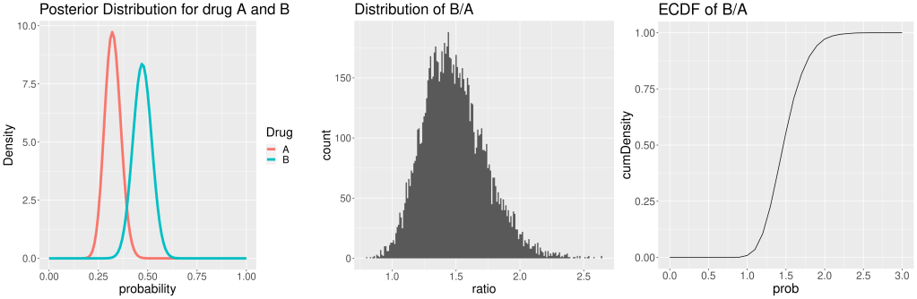
We will take a weak prior distribution of Beta(2, 8) for both drugs. And Beta(40, 80) for drug A, Beta(50, 50) for drug B as likelihood functions. The posterior distributions for both drugs are very easy to compute, that are Beta(42, 88) for drug A and Beta(52, 58) for drug B. The following procedures will be explained in the following R code.
From posterior distributions of A and B, we can see, probabilities of 5-year survival for B is in general bigger than for A, however there is an overlapping. Based on the random sampling, 99% of the time B is more effective than A. The histogram of differences between B and A shows that B is most likely about 50% more effective than A. Finally, ECDF indicates that it is almost impossible for drug A being more effective than drug B (B/A<1). Besides, there is about 50% probability drug B has 50% or more improvement than A.
library(tidyr)
library(ggplot2)
library(tibble)

## set up priors
prior.alpha=2
prior.beta=8

x=seq(from=0,to=1,by=0.01)

## set up posterior distributions for A and B in tibble, then plot
tibble(probability=x,
       A=dbeta(x,40+prior.alpha,80+prior.beta),
       B=dbeta(x,50+prior.alpha, 50+prior.beta)) %>%
  pivot_longer(-probability,names_to="Drug",values_to = "Density") %>%
  ggplot()+
  geom_line(aes(x=probability,y=Density,color=Drug),linewidth=2)+
  theme(text=element_text(size=21))+
  ggtitle("Posterior Distribution for drug A and B")

ggsave("plots/Bayesian_paraEsti_ABtest.png")

## set up random draws from posterior distributions of A and B
n=10000
sample.A=rbeta(n, 40+prior.alpha,80+prior.beta)
sample.B=rbeta(n,50+prior.alpha,50+prior.beta)

## caclulate in how many pair of randomw draws, B is better than A
sum(sample.B>sample.A)/n #99.13% time B is more effective than A

## calculate how many times B is than A
BA_ratio=data.frame(ratio=sample.B/sample.A)

ggplot(BA_ratio)+
  geom_histogram(aes(ratio),binwidth = 0.01)+
  theme(text=element_text(size=21))+
  ggtitle("Distribution of B/A")

ggsave("plots/BAratio.png")

## empirical cumulative density of the difference between B and A
ecdf_BAratio=ecdf(BA_ratio$ratio)
x=seq(0,3,by=0.1)

ggplot(data=tibble(prob=x,cumDensity=ecdf_BAratio(x)))+
  geom_line(aes(x=prob,y=cumDensity))+
  scale_x_continuous(n.breaks=6)+
  theme(text=element_text(size=22))+
  ggtitle("ECDF of B/A")

ggsave("plots/ecdf_BAratio.png")
