Bayesian Statistics for Beginner

Bayesian Statistics is about how to use data to update your belief. It is not about how to use data to prove or support your hypothesis. Bayesian statistics lets people to combine their prior knowledges with observations to disagree or update with their beliefs in a quantitative way. The core of Bayesian thinking is the Bayes theorem:

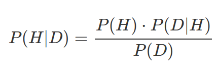
P(H): prior probability of your belief/hypothesis;
P(D|H): likelihood of observations given your hypothesis;
P(H|D): posterior probability of your hypothesis given the data;
P(D): probability of observations, in order to normalize posterior probability.

Bayes theorem can be derived by reversing the conditional probability P(D|H) to obtain P(H|D). We know P(H|D) can be calculated by the number of observation of both H and D divided by the observations of D. Assuming the total observation is N, then:

We can also derive this by P(H,D)=P(D,H), so P(H)P(D|H)=P(D)P(H|D), therefore we can get P(H|D)=P(H)P(D|H) / P(D).

We usually use probability distributions to present prior and likelihood, other than a single probability for each, to capture a wide range of possible believes. For instance, when we observe 2 times lottery wins among 10000 tries, we use Beta(2,9998) other than 0.0002 as a likelihood of winning lottery based on data we have. More about Beta Distribution will be in a future blog post.

Prior probability or prior distribution ( P(H) ) in Bayesian is the most controversial subject as many considers it to be subjective. However, they are vital as priors allow us to use background knowledge and past experiences to adjust the likelihood of data ( P(D|H) ). Prior distribution can be, objected by many Bayesian statisticians, chosen as “fair” or in other words “un-informal“, such as Beta(1,1) (everything is possible) or Beta(0,0) (everything is impossible). Alternatively, prior distribution can be informal but “weak“, such as Beta distribution with a smaller alpha and beta. Such priors can be helpful to avoid biased conclusion from observations where data points are few. Such “weak” priors are also easier to be “overridden” by actual data. Eventually when the amount of data grows, posterior distribution evolves to assemble the likelihood of data. In other word, when there are a lot of data, the posterior distribution shifts towards data without prior, and you shift your belief towards data (unless you hold an extremely strong prior belief!).

Best prior is always based on actual data. If you do not have data, Bayesian prior provides a quantitative way to measure and record your experience. Even if your prior beliefs were wrong, it is at least recorded in a quantitative way and can be overturned by data. There is no “fair” priors, when you know absolute nothing, it is better to admit that you can not conclude, other than using a “fair” prior that might result in an unrealistic posterior output.

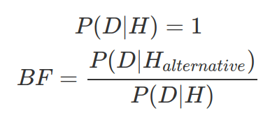
One core concept in Bayesian, and a great mental model, is that every belief should be falsifiable. Every belief should accept challenge. You can not adopt a belief that can not be proved wrong. This is extremely dangerous as such belief can be even strengthened by evidence contradicting to it. As shown below, if you consider given your belief, the probability for getting the data is always 100%. Then, the more data you observe, the more Bayes Factor will be in favour of your hypothesis (as the alternative Hypothesis is not absolute). For instance, your hypothesis is environmentalists are making up the data. And the alternative hypothesis may contain probability for global temperature increases per year (p). As the number of year (n) with increased temperature grows, the overall probability is actually decreasing (), resulting in smaller Bayes Factor, supporting your unrealistic hypothesis.

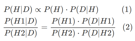
In real world, P(D) is often impossible to estimate. However, in many cases, we either approximate posterior distribution (1) or compare hypotheses (2), therefore we do not need to explicitly know P(D).