Binomial Distribution describes probabilities of getting a number of successful trials (variable, k) within a fixed total number of trials (constant parameter, n), given the probability of one successful trial is known and fixed (constant parameter, p) (B(k; n, p)). Each trial in binomial distribution, as described above, is a Bernoulli event that can only have two outcomes, success or failure. If there are more than two outcomes in each trial, it is not a binomial distribution but a multinomial distribution.
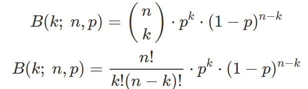
Each binomial probability describes the likelihood of getting k number of successes in the fixed n number of total trials. It does not care about the orders how these k successful events occur with the n-k number of failures. Binomial probability is simply calculated by multiplying the number of permutations (orders or combinations) of k number of successes in n events (Binomial Coefficient) with the probability of one such combination. The Probability Mass Function (PMF) of Binomial distribution is as following. The “mass” part indicates it computes probability for any given k. And the reason it is called “mass” other than “density” is because binomial is a discrete distribution.
Binomial coefficient 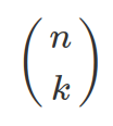 (pronounced as “n choose k”), can be computed in R by function
 choose(n,k). The explanation for why Binomial Coefficient is computed as above is to first assume n events gives n complete different outcomes. So the combinations of getting k number of outcomes from these n different outcomes are the factorial n!/(n-k)! (there are n options for the first event, then one less option for each proceeding events. For example, 5 choose 3, will give 5*4*3 different combination given 5 are all different options). However, in our case, the k number of events are all the same (successes) and we do not care about their orders. Therefore we need to remove all the repeats in above combinations. That is why we divide the above combinatorial by k! (the possible combinations of k number of success if they are different).
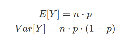
The mean (also called the expectation of data) and variance of a variable, Y, derived from Binomial distribution are:
The parameter p (probability of getting desirable outcome in each Bernoulli event) can be estimated from data. The estimation of p is 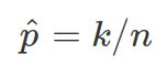 (as proportion of successes over all trials). This is also called the Maximum Likelihood Estimate (MLE) of the true parameter p. MLE is based on data at hand, and varies when sample size differs. However, when sample size n increases, the estimated p approximates real p. The likelihood function is shown below, the MLE estimates tries to find the p gives most likelihood for the data at hand (p will be between 0 and 1. However this way of estimation used data twice, once for estimate, once for evaluation.).
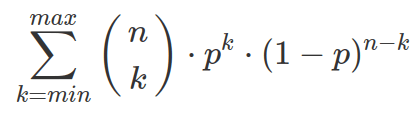
Binomial distribution is discrete, so you can not “integrate” ( ) the PMF over a range of k values. In stead, you need to sum each individual probability corresponding to a specific k together (or use CDF for binomial in R).
Useful R functions:
Binomial Probability Mass Function (PMF): dbinom(k, n, prob)
Binomial Cumulative Distribution Function (CDF): pbinom(k, n, prob, lower.tail=TRUE). By default, this compute probability of obtaining k or less than k success events (k is inclusive). When use pbinom(k, n, prob, lower.tail=FALSE), this computes probability of obtaining more than k successes(k is not included).
Binomial Quantile Function (reverse of CDF): qbinom(p, n, prob, lower.tail=TRUE), this computes the probability (p) corresponds to obtaining k or less than k successes.
R
# binomial coefficient
> choose(n=3,k=2)

# binomial PMF
> dbinom(2,3,0.5) #the probability of getting two heads in 3 coin tossings.

# sum binomial PMF over a range of k
> pbinom(2,3,0.5,lower.tail=TRUE) #probability of getting 2 or less than 2 heads in 3 coin tossing

# quantile
> qbinom(0.5,3,0.5,lower.tail=TRUE) #what is the max number of heads I can get half of the time of coin tossing.