Probability captures how strong, or how uncertain, we believe in the world. It is a natural extension of logic (absolute believes, binaries). The probability for an event to occur lies between 0 and 1 (rule No.1). Probability can be calculated as the proportion of number of desirable events over the total number of events. For instance, the probability of getting a six from a six-sided dice, can be calculating by how many times you get six from 10 throws.
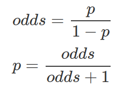
Some times, we express how strongly we believe in something as Odds (note this is different from Odds Ratio, which measures the association between event A and B). Odds are calculated as the ratio between the number of events produce the desirable outcome over the number of events does not. Therefore, from odds we can calculate the probability of getting the desirable outcome:
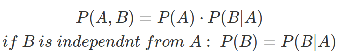
Probabilities can be combined by AND relation. For instance, we can calculate the probability of A event AND B event both occur by:
Two events are independent if and only if the probability of both events occurring is P(A)P(B) (rule No.2).
When combining more than two probabilities by AND relation (based on my understanding):

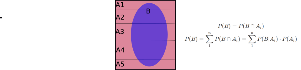
When event B is the intersection of B with n dis-joint probabilities across all the sample space, A, shown as following. Then P(B) equals to joint probability of B and each A, weighted by P(Ai):
Probabilities can also be combined by OR relation. For instance, we can calculate the probability of A event OR B event occurs by (rule No.3):

Probability Distribution describes probabilities for a whole range of situations other than just for one situation. The probabilities of all possible events in the entire sample space must sum up to 1 (rule No.4).
In general, we assume the data we observed, y, are generated from a random variable Y, which is considered as the function to “project” possible outcomes from sample space, S, to real number system. Y: S -> R. Y can have parameters, such as ![]() , and Probability Mass Function (PMF, for discrete probability distribution) or Probability Density Function (PDF, for continuous probability distribution), written as p(y|
, and Probability Mass Function (PMF, for discrete probability distribution) or Probability Density Function (PDF, for continuous probability distribution), written as p(y|![]() ).
).
When we assume variable Y is from, for instance, Binomial distribution or any other distribution, we use the following annotation: 
Bayesian statistics ask how uncertain about ![]() and treat it as a variable by assigning probability distribution to it p(
and treat it as a variable by assigning probability distribution to it p(![]() ), which is called prior distribution on
), which is called prior distribution on ![]() . And p(y|
. And p(y|![]() ) is likelihood, p(
) is likelihood, p(![]() |y) is posterior distribution.
|y) is posterior distribution.
